MiMo-V2.6: Groupwise Grading, Frozen Routers, and RL at 25K Sequences per Step
Reading notes on:
The MiMo-V2.6 report is mostly about RL at scale on long-horizon, agentic, omni-modal tasks. The architecture section is competent and brief. The substance is in how the RL is fed, graded, regularized, and kept from falling over. Two MoE models:
| Total params | Active params | Experts (active) | Layers | |
|---|---|---|---|---|
| MiMo-V2.6-Pro | 1.02T | 42B | 384 (8) | 70 |
| MiMo-V2.6-Flash | 310B | 15B | 256 (8) | 48 |
RL compute is scaled along three independent axes:
- Throughput: 1,568 prompts × 16 rollouts $\approx$ 25K sequences per step, or 2.7B–3.7B tokens per update.
- Environments and harnesses: heterogeneous tasks, with agents run under many different scaffolds.
- Grading: groupwise, agentic reward and advantage shaping that goes beyond binary pass/fail.
The sections below follow that order: backbone, objective, grading, regularizers, infrastructure, results.
1. Architecture and Pre-/Mid-Training
Hybrid-SWA backbone
The text backbone stacks $M$ hybrid blocks. Each block is $N$ local sliding-window attention layers (window $W = 128$) followed by one global attention layer:
\[\text{Hybrid Block} = \Big[ \underbrace{\text{SWA} \to \cdots \to \text{SWA}}_{N \text{ layers}} \to \text{GA} \Big]\]- Pro: 60 SWA + 10 GA = 70 layers. Flash: 39 SWA + 9 GA = 48 layers.
- The first block uses global attention with a dense FFN, for representation stability.
A 128-token window is very aggressive. Most of the KV cache is effectively constant-size, and the long-range work falls to a handful of GA layers. That is the same bet as the hybrid attention in DeepSeek-V4 and the aggressive KV compression in DeepSeek-V4.1-Flash: long-horizon agents are bound by KV memory, so architects keep cutting it.
DFlash instead of MTP
MiMo-V2.6 replaces standard multi-token prediction with a 5-layer DFlash block-diffusion drafter. It runs over an SWA context of 1,024 and predicts 7 draft tokens in parallel per forward pass, giving +31.3% accepted draft length during RL rollouts. The rollout-side number is the one that matters. In agentic RL, generation dominates wall-clock time, so a better drafter translates directly into more RL steps.
Omni-modal encoders
- MiMo-ViT (681M, 28 layers): sink-augmented SWA that alternates between row-major and column-major token serialization, so spatial information crosses window boundaries without quadratic global attention. Periodic GA layers aggregate global context.
- Audio: a 308M audio tokenizer (12 SWA + 12 GA layers) over log-mel spectrograms, with a 20-layer residual vector quantizer producing 20 discrete tokens at 25 Hz. A 127M audio patch encoder groups every 4 frames, taking the token rate from 25 Hz down to 6.25 Hz.
Muown and MXFP4 QAT in mid-training
Pre-training covers text, vision, and audio (48T tokens for Flash, 30T for Pro). In mid-training the hidden weight matrices move from AdamW to Muown, the authors’ variant of Muon with explicit row-norm control. It removes spectral-norm drift and reduces sensitivity to weight decay. The stated motivation is that AdamW’s efficiency degrades at the batch sizes RL will use.
- Embeddings, LM heads, and MoE routers stay on AdamW. Hidden matrices use Muown.
- Mid-training also includes MXFP4 quantization-aware training, conditioning the weights for low-precision inference in RL rollouts. This is the same move as FP4 QAT in DeepSeek-V4’s infra, and the train/rollout precision question from NVFP4 in the RL loop handled upstream.
2. The RL Objective
Training uses GRPO with asynchronous partial rollouts. For a prompt $q$ from the task mixture $\bigcup_d \mathcal{D}_d$, the rollout policy $\mu_{\theta_{\text{old}}}$ samples $G = 16$ trajectories $\{o_i\}_{i=1}^G$:
\[L(\theta) = -\mathbb{E}_{q,\, \{o_i\} \sim \mu_{\theta_{\text{old}}}} \left[ \frac{1}{\sum_{i=1}^G \lvert o_i \rvert} \sum_{i=1}^G \sum_{t=1}^{\lvert o_i \rvert} r_{i,t}\, M_{i,t}\, A_{i,t} \log \pi_\theta(o_{i,t} \mid q, o_{i,<t}) \right]\]- $r_{i,t} = \text{sg}\left[\frac{\pi_\theta(o_{i,t})}{\mu_{\theta_{\text{old}}}(o_{i,t})}\right]$ is a stop-gradient token-level importance ratio. It weights a plain $\log\pi$ gradient instead of being differentiated through the way the PPO ratio is.
-
$M_{i,t}$ is a clip mask with decoupled bounds for positive and negative advantages:
\[M_{i,t} = \mathbf{1} \left[ \left( A_i \ge 0 \wedge \epsilon_l^+ \le r_{i,t} \le \epsilon_h^+ \right) \vee \left( A_i < 0 \wedge \epsilon_l^- \le r_{i,t} \le \epsilon_h^- \right) \right]\]The bounds are initialized to $[0.2, 5.0]$ and adjusted dynamically based on online policy entropy.
- Prompt-mean aggregation. The normalizer $\sum_i \lvert o_i \rvert$ is per group, and groups are then averaged. Each prompt carries equal weight, rather than every token in the global batch. Global token normalization gives long responses a larger share of the gradient, which lets length run away. Prompt-mean aggregation removes that incentive.
Masking tokens outside the trust region (rather than clipping the ratio and letting gradient flow at the boundary) plus a detached IS weight is a clean way to handle the off-policy gap that asynchronous rollouts create. Score centering looks at a different component of the same problem.
3. Groupwise Agentic Grading
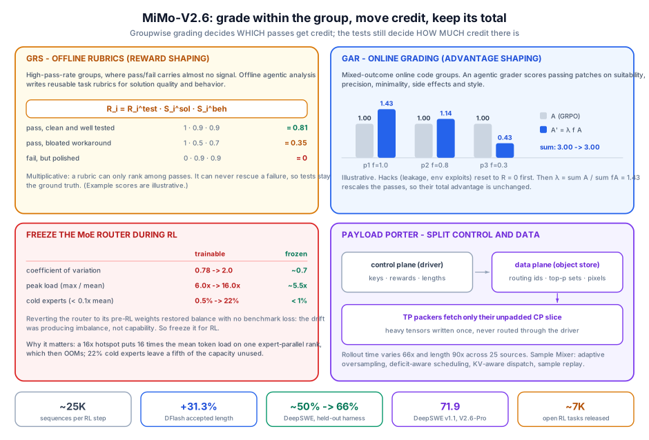
Binary pass/fail gives the same reward to a concise, correct patch and a bloated workaround that happens to pass. MiMo-V2.6 adds two groupwise schemes for different regimes.
3.1 Groupwise Reward Synthesis (GRS): offline rubrics
For high-pass-rate tasks, where most of the group passes and pass/fail carries almost no signal, an offline agentic analysis produces reusable task-specific rubrics. They score solution quality $S^{\text{sol}} \in (0,1]$ and problem-solving and verification behavior $S^{\text{beh}} \in (0,1]$:
\[R_i = R_i^{\text{test}} \cdot S_i^{\text{sol}} \cdot S_i^{\text{beh}}\]The multiplicative form is the design choice. A failing trajectory ($R^{\text{test}} = 0$) stays at zero however polished it looks. A rubric can only rank among passes. It can never rescue a failure, so tests remain the ground truth.
3.2 Groupwise Advantage Redistribution (GAR): online grading
For online code tasks with mixed-outcome groups, an agentic grader reviews the passing patches along five dimensions: approach suitability, implementation precision, minimality, absence of side effects, and consistency with the codebase style.
- Hack correction. Trajectories showing solution leakage or environment exploitation have their reward reset to $R_i = 0$.
- Advantage redistribution. For the passing set $\mathcal{P} = \{i : R_i = 1\}$, quality factors $f_i \in (0,1]$ down-weight weaker passes, and a scalar $\lambda$ returns the removed mass to the stronger ones:
By construction $\sum_{i \in \mathcal{P}} A_i’ = \sum_{i \in \mathcal{P}} A_i$. The group’s net positive advantage is unchanged. What changes is which passes receive it. An illustrative example: three passes at $A = 1$ with $f = (1.0, 0.8, 0.3)$ give $\lambda = 3/2.1 \approx 1.43$ and $A’ \approx (1.43, 1.14, 0.43)$, which still sums to 3.
The two schemes differ on purpose. GRS changes rewards, which suits groups where nearly everything passes and there is no advantage to redistribute. GAR changes advantages and conserves their mass, so the pass/fail signal in mixed groups keeps its scale and quality only decides how it is split. It is a coarse, group-level form of the credit-assignment problem in Le Critique.
4. Behavioral Regularization and Stability
4.1 Group-relative length penalty
To stop the policy from padding its reasoning to raise pass probability, groups above a pass-rate threshold get a length penalty relative to their own successful rollouts:
\[\ell_q^\star = \text{Quantile}_{B/100} \{\ell_j : j \in \mathcal{P}_q\}\] \[\tilde{R}_i = R_i - \mathbf{1}[i \in \mathcal{P}_q] \cdot X \cdot \left[ \text{clip}\left( \frac{\ell_i / \ell_q^\star - 1 - \delta}{s - \delta}, 0, 1 \right) \right]^\gamma\]- $\ell_i = \lvert o_i \rvert$. The target $\ell_q^\star$ is the $B$-th percentile length among passing rollouts.
- $X \ge 0$ is the maximum deduction, $\delta$ the relative excess that is tolerated for free, $s$ the saturation point, and $\gamma \ge 1$ the exponent.
Only passing rollouts are penalized, and only for exceeding what their passing peers needed. The reference is per prompt, so a hard problem that genuinely needs 40K tokens is not penalized for being hard.
4.2 Segment-level behavioral penalties
Malformed XML or an invalid tool argument partway through an otherwise good trajectory should not zero the whole trajectory. Let $h_{i,t} \in \{0,1\}$ flag offending tokens:
\[A_{i,t} = \begin{cases} \alpha (1 - h_{i,t}) A_i, & A_i > 0 \\ \big[ \beta (1 - h_{i,t}) + \kappa h_{i,t} \big] A_i, & A_i < 0 \\ 0, & A_i = 0 \end{cases}\]In positive trajectories, flagged tokens get no credit. In negative trajectories they get an amplified penalty ($\kappa > 1$). The scalars $\alpha, \beta$ conserve advantage mass over the unflagged tokens $C^\pm$:
\[\alpha = \min \left( \alpha_{\max}, 1 + \frac{\sum_{H^+} A_i}{\sum_{C^+} A_i} \right), \quad \beta = \max \left( \beta_{\min}, 1 - \frac{(\kappa - 1) \sum_{H^-} \lvert A_i \rvert}{\sum_{C^-} \lvert A_i \rvert} \right)\]This is the same conservation principle as GAR, applied to tokens instead of trajectories: move credit around, keep its total fixed.
4.3 Freeze the router
For MoE engineers, this is probably the most useful finding: trainable routers suffer severe load collapse during RL.
| Metric | Trainable router, start → end of RL | Frozen router |
|---|---|---|
| Coefficient of variation | 0.78 → 2.0 | $\approx$ 0.7 |
| Peak load (max / mean) | 6.0× → 16.0× | $\approx$ 5.5× |
| Cold-expert fraction (< 0.1× mean) | 0.5% → 22% | < 1% |
A 16× hotspot means one expert-parallel rank gets 16 times the average token load, which leads to OOM. 22% cold experts means a fifth of the capacity is starved. The key experiment: restoring the router weights to their pre-RL values restored load balance without hurting benchmark scores. The router drift was producing imbalance without adding capability. So the router is frozen for RL, load metrics stay flat, and the expert-parallel OOMs disappear.
This is a blunter fix than Rollout Routing Replay, which keeps the router trainable but aligns training-time routing with inference-time routing. It also makes the placement problem in RoutePack and UltraEP much easier: a frozen router’s load distribution is stationary.
5. Agent Infrastructure: Sample Mixer and Payload Porter
5.1 Sample Mixer for heterogeneous rollouts
Across 25 task sources, mean rollout time varies 66× and generated length varies 90×. A naive synchronous batch waits on the slowest source. This is the trainer/generator mismatch from RL Systems Mind the Gap, made worse by agentic variance. The Sample Mixer uses four mechanisms:
-
Adaptive rollout concurrency. Oversampling ratios $p_i$ are set from each task’s active duration $t_i$, acceptance rate $r_i$, and target batch share $B_i$:
\[p_i = \text{clip}(c\, t_i - 1, p_{\min}, p_{\max}), \quad \text{s.t. } \frac{\sum_i m_i p_i}{\sum_i m_i} = \bar{p}\] -
Adaptive rollout scheduling. Prompt weights blend long-run demand with the current deficit:
\[w_i = \alpha \frac{B_i}{r_i} + (1 - \alpha) \frac{(B_i - A_i)_+}{r_i}\] - Predictive rollout dispatch. New rollouts go to GPU ranks according to remaining KV-cache memory and estimated inference concurrency.
- Sample replay. On startup or recovery, completed rollout groups from slow sources are reused so they do not stall collection.
5.2 Payload Porter: separate control and data planes
At tens of thousands of long-context trajectories, each carrying MoE routing indices, top-$p$ candidate sets, and screenshots, the driver node runs out of memory. MiMo-V2.6 splits the two planes:
- Control plane: only lightweight scalar metadata (keys, rewards, context lengths).
- Data plane: heavy tensors are written once to a distributed object store. At training time, tensor-parallel packers fetch only the unpadded context-parallel slices their rank needs.
The same principle, keeping bulk state off the coordinator, appears on the sandbox side of agentic RL in DeepSeek’s DSec. There, rollout state lives on the sandbox platform instead of the preemptible GPU pod.
6. Results and Open Releases
| Benchmark | Metric | V2.6-Flash | V2.6-Pro | Claude Opus 5 | GPT-5.6 Sol |
|---|---|---|---|---|---|
| Code: DeepSWE v1.1 | pass@1 / avg@3 | 67.9 | 71.9 | 74.0 | 73.0 |
| General: AutomationBench v1.0.6 | avg@1 | 52.3 | 53.1 | 50.3 | 45.8 |
| General: OSWorld-Verified | avg@1 | 80.8 | 82.0 | 83.4 | 83.0 |
| Cyber: CyberGym | avg@3 | 95.1 | 94.0 | not reported | not reported |
| Visual: MiMo Visual Coding | avg@1 | 71.5 | 72.3 | 70.0 | 73.4 |
Pro trails the closed frontier by 2–3 points on DeepSWE and about 1 on OSWorld, leads on AutomationBench, and Flash stays close to Pro throughout.
Multi-harness cross-transfer
Training across modular, decoupled mini-harnesses raised the average DeepSWE v1.1 pass rate on held-out production harnesses (Codex, Claude Code, mini-swe-agent) from ~50% to 66%. A policy trained under a single scaffold overfits to that scaffold’s prompts and tool wrappers, and harness diversity is the fix. This fits the harness-sensitivity results in HarnessDev and Meta-Harness: the harness is part of the environment, and RL should randomize over it.
Open-source suite
- MiMo-V2.6-Distill-Qwen-9B: an SFT checkpoint distilled on 77.4B tokens of agentic trajectories.
- Open RL environments: ~7K curated tasks across code, cyber, general workflows, and visual web development, with automated verifiers.
- An end-to-end RL framework, including the mini-harnesses and groupwise grading tools.
Takeaways
- Shape advantages without changing their total. GAR (across trajectories) and segment penalties (across tokens) both move credit toward better behavior while keeping the net signal fixed. The rubric decides how credit is split. The tests decide how much there is.
- Keep tests as a multiplicative gate. $R^{\text{test}} \cdot S^{\text{sol}} \cdot S^{\text{beh}}$ means no rubric score can turn a failure into a success.
- Freeze the MoE router for RL. Drift during RL produced load collapse (CV 0.78 → 2.0, 22% cold experts) and no capability, and reverting it cost nothing.
- Prompt-mean aggregation, group-relative length targets. Both remove the gradient’s preference for long outputs without penalizing problems that are genuinely hard.
- Randomize the harness. Multi-harness RL took held-out-harness DeepSWE from ~50% to 66%.
- At 25K sequences per step, the infrastructure is part of the algorithm. Oversampling, deficit-aware scheduling, KV-aware dispatch, and separate control and data planes are what make the step size workable.