RoutePack: Joint Expert Placement and Attention-Aware Packing for MoE RL
Reading notes on:
MoE RL has two different max operators fighting each other.
- On the dense side, a data-parallel microbatch is paced by its longest or most quadratic sequence.
- On the sparse side, an expert-parallel layer is paced by the busiest physical rank receiving routed tokens.
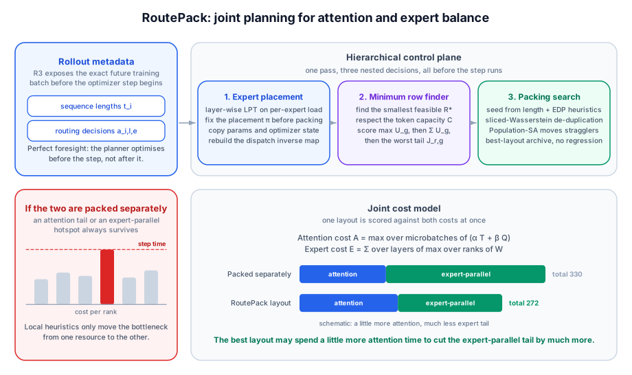
If you optimize only one, you often make the other worse. That is the systems “whack-a-mole” at the heart of RoutePack. The paper’s key insight is that RL gives you something pretraining does not: with R3-style routing replay, the training step already knows the future sequence lengths and expert routes of the rollout batch. So the batch planner can solve attention packing and expert placement jointly, before the optimizer step begins.
1. The Bottleneck Is Joint by Construction
In RL post-training, moving one sample $S_i$ to a different slot changes three things at once:
- its sequence-length contribution inside the data-parallel microbatch;
- its quadratic token-pair term for MLA or MHA attention;
- its layer-wise expert demand on physical expert-parallel ranks.
That coupling is why “pack by length first, balance experts later” fails. You may reduce dense attention tails and simultaneously create a disastrous expert hotspot. Conversely, spreading expert traffic can make attention far less regular.
This is the same family of problem that UltraEP solves inside a single MoE layer, except here the optimization lives one level up: the scheduler is rearranging whole sequences across the RL batch.
2. RL Gives the Planner Perfect Foresight
Because rollout and training consume the same token sequences, the planner gets the exact metadata for each sample:
\[\{(t_i, A_i)\}_{i=1}^N, \qquad A_i = [a_{i,l,e}]_{l \in \mathcal{L}_{MoE}, e \in \mathcal{E}_l},\]where $t_i$ is the response length and $a_{i,l,e}$ counts how many tokens in sample $i$ hit logical expert $e$ at MoE layer $l$.
Once a layer-wise expert map $\pi_l$ is fixed, the demand of sample $i$ on physical rank $p$ at layer $l$ becomes
\[q_{i,l,p}(\pi_l) = \sum_{e:\,\text{owner}(\pi_l(e)) = p} a_{i,l,e}.\]For row $r$ and EDP shard $g$, the routed-token load on physical rank $p$ is
\[W_{r,g,l,p}(\pi, x) = \sum_{d \in \mathcal{D}_g} \sum_{i=1}^N x_{i,r,d}\, q_{i,l,p}(\pi_l).\]The row-level expert cost is then the sum of peak loads over MoE layers:
\[E_{r,g} = \frac{1}{C} \sum_{l \in \mathcal{L}_{MoE}} \max_p W_{r,g,l,p}(\pi, x).\]RoutePack models dense attention with a calibrated linear-quadratic proxy:
\[F_A(B_{r,d}) = \alpha_s T_{r,d} + \beta_s Q_{r,d},\]where
\[T_{r,d} = \frac{1}{C}\sum_{i \in B_{r,d}} t_i, \qquad Q_{r,d} = \sum_{i \in B_{r,d}} \left(\frac{t_i}{C}\right)^2.\]This matters because the hybrid attention stacks in real MoE RL systems mix linear-style layers like KDA with quadratic components, so a pure length heuristic is not enough.
The total row-local projected cost is
\[J_{r,g} = A_{r,g} + E_{r,g}.\]That is the quantity the planner is actually trying to minimize.
3. The Objective Is Lexicographic, Not Scalar
RoutePack first finds the minimum feasible row count $R^*$ under token capacity $C$:
\[R^* = \min \{R : \mathcal{X}_R \ne \emptyset\}.\]That prevents the planner from “cheating” by adding rows and lowering peaks at the cost of higher end-to-end latency.
With $R^*$ fixed, the sequence layout $x$ is optimized under the tuple
\[\text{Score}(x; \pi) = \left( \max_g U_g,\; \sum_g U_g,\; \max_{r,g} J_{r,g} \right),\]where $U_g = \sum_r J_{r,g}$ is the total projected work of shard $g$.
The ordering matters:
- minimize the slowest shard’s total work;
- then minimize total work across shards;
- then minimize the single worst row-local tail.
This is the right design for training systems. It optimizes both wall-clock stragglers and cluster waste without letting one wash out the other in an arbitrary scalar weighting.
4. The Three-Stage Planner
Jointly optimizing expert map and packing would be intractable, so the system splits into a control plane and a data plane.
4.1 Layer-wise LPT expert placement
For each MoE layer $l$, aggregate expert demand
\[L_{l,e} = \sum_i a_{i,l,e},\]sort experts by descending load, then place them with Longest Processing Time (LPT) onto physical ranks with open slots. This is greedy, but it does the important job: flatten the global expert map before any row-level packing begins.
The clever part is how the map is committed at runtime. RoutePack does in-place parameter and optimizer-state copies into pre-allocated physical slots and applies the inverse permutation in dispatch. It does not rebuild the execution graph or parameter objects. That makes expert remapping compatible with standard Megatron-style training stacks such as Megatron Core MoE.
4.2 Diverse seeding plus quality-diversity filtering
Under fixed $R^*$ and $\pi$, the search space is still nasty. RoutePack generates a population of diverse seeds using:
- window shuffle over length-sorted samples;
- randomized best fit over candidate cells;
- EDP-aware pairing that explicitly looks at expert-peak increments.
It then removes near-duplicates using a Sliced-Wasserstein sketch over row feature matrices. The sort-based sketch is row-permutation invariant, which avoids expensive Hungarian matching and keeps the planner fast enough to run online.
4.3 Population annealing
The filtered seeds are improved with Population-SA: multiple MCMC chains, guided swap proposals, systematic resampling, and a best-layout archive that guarantees non-regression. The scalar search energy is just a tight encoding of the lexicographic score:
\[\mathcal{E}(x) = s_0(x) + 10^{-6}s_1(x) + 10^{-9}s_2(x).\]The resampling is what makes the method more than “simulated annealing with restarts.” Good layouts are cloned; bad ones die off; the global best is preserved outside the resampling path.
5. Why the Planner Can Be Free
RoutePack overlaps planning with model-state materialization on the actor side. Let
- $T_{LPT}$ be expert-reordering time;
- $T_{pack}$ be packing-search time;
- $T_{actor}$ be placement-aware model-state materialization;
- $T_{aux}$ be other runtime preparation.
The key condition is
\[T_{LPT} + T_{pack} \le \max(T_{LPT}, T_{aux}) + T_{actor}.\]If that inequality holds, then the entire CPU-side planning cost disappears under the already-required GPU-side state movement. That is a very practical result: a sophisticated scheduler is only useful if it does not itself become the new bottleneck.
6. The Payoff
RoutePack is evaluated on two GRPO workloads over GSM8K:
| Model | Baseline tokens/s | LPT only | RoutePack | Net gain |
|---|---|---|---|---|
| Ling-3.0-Tiny | 42.86 | 44.49 | 46.65 | +8.85% |
| Ling-3.0-Flash | 68.50 | 75.69 | 78.70 | +14.89% |
The nicest detail is how the gain happens. Relative to length-only packing, RoutePack willingly accepts a tiny attention penalty:
- Tiny: attention cost +0.09%
- Flash: attention cost +0.77%
in order to cut the worst expert tails much more:
- Tiny: worst row/layer EP peak -11.04%
- Flash: worst row/layer EP peak -11.62%
That trade lowers the joint projected cost by 1.53% and 1.35% respectively, which is enough to move end-to-end throughput materially.
This is the main systems lesson of the paper: component-wise monotonic improvement is the wrong objective. The optimal batch layout may make one subsystem slightly worse in order to make the combined pipeline substantially better.
Takeaways
- Never optimize MoE RL in silos. Dense attention packing and sparse expert balance are coupled through the batch layout.
- R3-style replay is more than a stability fix. It exposes the exact route metadata the scheduler needs for closed-loop planning.
- The right objective is lexicographic. Row count, slowest shard, total work, and worst tail are not interchangeable.
- A little extra attention work can be the right trade. What matters is the joint pipeline maximum, not whether every subsystem improves in isolation.
- Scheduler sophistication only matters if it is hidden. RoutePack’s overlap story is as important as its optimization story.