Score Centering: Cancelling the Drift Term in Off-Policy RL
Reading notes on:
Everybody running LLM RL at scale has hit this. The sampler and the trainer are the same model (same weights, same architecture), and the run collapses anyway. You quantize the sampler to FP8 for throughput, or you let rollouts lag a few steps behind the weights, and reward goes to zero. The usual response is to reach for importance sampling, clip the ratios, and hope.
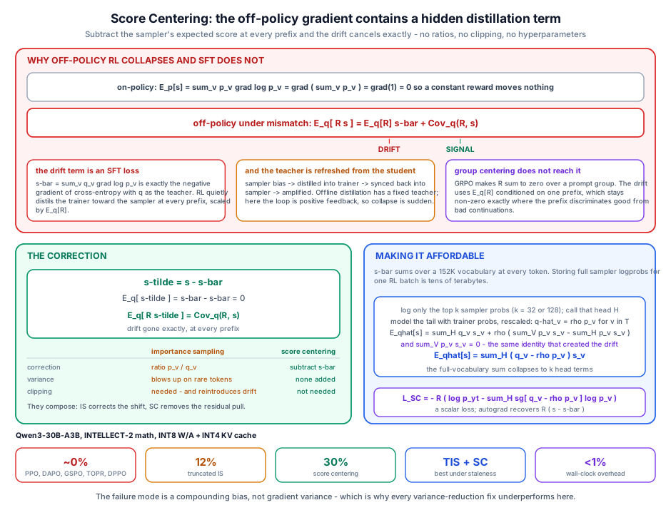
This paper explains what is actually going wrong, and it is not variance. Decompose the expected policy gradient under a mismatched sampler and it splits cleanly into two terms: a signal term you want, and a drift term that is a disguised distillation loss pulling the trainer toward the sampler’s numerical errors. Because the sampler gets refreshed from the trainer, that pull compounds. The fix, Score Centering, is one subtraction, has no hyperparameters, and costs under 1% wall clock.
1. Where the Mismatch Comes From
Policy gradient assumes rollouts come from the current training policy, $q_\theta = p_\theta$. Three things break that in any real system:
- Quantization. Samplers run FP8/INT8/INT4 to hit throughput targets; trainers run BF16 or FP32. Same weights, different arithmetic; see the NVFP4 RL loop and Jet-RL’s precision mismatch for what that looks like in practice.
- Non-associative floating-point reduction. This one gets mismatch even at identical precision. Decode emits one token at a time; training processes the sequence in parallel. Different reduction orders over the same values give different sums, because floating-point addition is not associative. Identical weights, identical kernels, different logits: the same effect catalogued in Training-Inference Parity in MoE Models.
- Staleness. Asynchronous and disaggregated RL serving delivers rollouts from checkpoints several steps old.
The puzzle the paper opens with is a good one: SFT does not care. You can fine-tune on data from a different model, an older checkpoint, a different tokenizer, and it works. Online RL under the same amount of distribution mismatch collapses. Why is RL uniquely fragile here?
2. The Drift/Signal Decomposition
Fix a prefix $y_{<t}$ and look at the expected update at that single position.
- $p_v = p_\theta(v \mid y_{<t})$, $q_v = q_\theta(v \mid y_{<t})$: trainer and sampler next-token probabilities.
- $s_v = \nabla_\theta \log p_v$: the score of token $v$ under the trainer.
- $\bar{s} = \mathbb{E}_{y_t \sim q}[s_{y_t}] = \sum_{v} q_v s_v$: expected score under the sampler.
- $R$: advantage/reward for the rollout.
On-policy, the expected score is exactly zero. This is the identity everything rests on:
\[\mathbb{E}_{p}[s_{y_t}] = \sum_{v} p_v \nabla_\theta \log p_v = \sum_v \nabla_\theta p_v = \nabla_\theta \sum_v p_v = \nabla_\theta(1) = 0\]So with a constant reward, no learning signal at all, the expected update is $R \cdot 0 = 0$. The algorithm does nothing when it has nothing to learn, which is the property you want.
Off-policy, it is not zero. With $y_t \sim q_\theta$ the sum is $\bar{s} \ne 0$ in general. Apply $\mathbb{E}[AB] = \mathbb{E}[A]\mathbb{E}[B] + \text{Cov}(A,B)$:
\[\mathbb{E}_q[R\, s_{y_t}] = \underbrace{\mathbb{E}_q[R]\,\bar{s}}_{\text{drift}} + \underbrace{\text{Cov}_q(R, s_{y_t})}_{\text{signal}}\]The second term is the learning: it moves the policy toward tokens whose reward exceeds the local average. The first term is new, and it has an identity.
2.1 The drift term is a distillation loss
$\bar{s} = \sum_v q_v \nabla_\theta \log p_v$ is exactly the negative gradient of the cross-entropy loss $-\sum_v q_v \log p_v$: the SFT loss with $q_\theta$ as the teacher. So the drift term makes the trainer distill toward the sampler, at every prefix, scaled by $\mathbb{E}_q[R]$.
That single observation answers the opening puzzle. SFT tolerates a mismatched data source because it has no such term. RL has an unrequested distillation objective bolted onto its gradient, and the teacher is a numerically corrupted copy of the student.
2.2 Why it compounds
In offline distillation a fixed teacher means a bounded error. Here the sampler is periodically re-synced from the trainer:
sampler bias → distilled into trainer → trainer synced back into sampler → bias amplified
A positive feedback loop. Each cycle the bias is reinforced rather than corrected, and the run walks itself off a cliff. This is why collapse is often sudden rather than gradual: the dynamics are multiplicative.
2.3 Why group centering does not save you
The natural objection: GRPO already centers advantages within a group, so $\mathbb{E}[R] = 0$, so the drift term vanishes. It does not, and the reason is a scope error.
Group centering makes rewards sum to zero over a prompt’s rollout group. The drift term involves $\mathbb{E}_q[R]$ conditioned on a specific prefix $y_{<t}$. Those are different expectations. A prefix that leads to correct completions has positive conditional expected reward; a prefix down a wrong path has negative. Both are non-zero.
And they are non-zero in exactly the wrong places. The prefixes where $\mathbb{E}_q[R \mid y_{<t}]$ deviates most from zero are the prefixes that discriminate good from bad continuations: the prefixes carrying the learning signal. Drift is largest precisely where the signal lives.
3. Score Centering
Restore the on-policy property by construction. Define the centered score:
\[\tilde{s}_{y_t} = s_{y_t} - \bar{s} = \nabla_\theta \log p_\theta(y_t \mid y_{<t}) - \sum_{v} q_v \nabla_\theta \log p_v\]Under the sampler,
\[\mathbb{E}_q[\tilde{s}_{y_t}] = \mathbb{E}_q[s_{y_t}] - \bar{s} = \bar{s} - \bar{s} = 0\]which is the exact analogue of the on-policy identity in §2, now holding under $q$ instead of $p$. Substituting back:
\[\mathbb{E}_q[R\,\tilde{s}_{y_t}] = \mathbb{E}_q[R]\underbrace{\mathbb{E}_q[\tilde{s}_{y_t}]}_{=\,0} + \text{Cov}_q(R, \tilde{s}_{y_t}) = \text{Cov}_q(R, s_{y_t})\]Drift is gone: exactly, at every prefix, not approximately or in expectation over a batch. The update is the pure reward–score covariance under $q$. (The covariance is unchanged by the centering, since $\bar{s}$ is a constant given the prefix.)
Two things make this nicer than it looks. It is additive, so it does not touch probability ratios at all, and $\bar{s}$ is deterministic given the prefix (it is a sum over the vocabulary, not a sampled quantity), so subtracting it adds no estimator variance.
3.1 Against importance sampling
| Importance sampling (IS / TIS / MIS) | Score centering | |
|---|---|---|
| Correction | Multiplicative ratio $r_v = p_v / q_v$ | Additive subtraction $\tilde{s} = s - \bar{s}$ |
| Variance | Inflates on rare tokens where $q_v$ is small | Deterministic given prefix; no ratio variance |
| Clipping | Required in practice, and clipping reintroduces drift | None needed |
| Token dropping | Masking discards tokens | Keeps every token |
| Composition | The baseline | Composes cleanly with IS |
The clipping row is the sharp one. Clipping exists to control IS variance, but a clipped ratio is a biased estimate, and the bias is the drift you were correcting for. The standard fix quietly reintroduces the disease.
They are also not competitors. IS corrects a distributional shift between $p$ and $q$; SC removes a systematic pull toward $q$. When both are present (and under staleness they are), you want both.
4. Making It Cheap
The obvious problem: $\bar{s} = \sum_{v \in \mathcal{V}} q_v s_v$ is a sum over a 152K-token vocabulary at every position. Storing full sampler logprobs for an RL batch is tens of terabytes. Dead on arrival unless you can approximate it.
4.1 Top-$k$ tail reconstruction
Log only the top-$k$ sampler probabilities ($k = 32$ or $128$), call that head set $H$, tail $T$. Model the unlogged tail with trainer probabilities rescaled to match the sampler’s leftover mass:
\[\rho = \frac{1 - \sum_{v \in H} q_v}{1 - \sum_{v \in H} p_v}, \qquad \hat{q}_v = \begin{cases} q_v & v \in H \\ \rho\, p_v & v \in T \end{cases}\]Now compute the expected score under $\hat q$, and watch the tail eliminate itself:
\[\mathbb{E}_{\hat{q}}[s] = \sum_{v \in H} q_v s_v + \rho \sum_{v \in T} p_v s_v = \sum_{v \in H} q_v s_v + \rho\Big(\underbrace{\textstyle\sum_{v} p_v s_v}_{=\,0} - \sum_{v \in H} p_v s_v\Big) = \sum_{v \in H} (q_v - \rho\, p_v)\, s_v\]The step that makes it work is reusing the on-policy identity from §2: $\sum_v p_v s_v = 0$ exactly, so the unknown tail sum $\sum_{v \in T} p_v s_v$ can be rewritten as $-\sum_{v \in H} p_v s_v$, which is over the head and therefore known. The full-vocabulary sum collapses to $k$ terms with no approximation beyond the tail-shape assumption. That is an elegant piece of algebra: the same identity that created the problem is what closes it.
4.2 As a scalar loss
You do not need custom gradient code. Score centering is a scalar loss an autograd engine differentiates correctly on its own:
\[\mathcal{L}_{SC} = -R\left(\log p_{y_t} - \sum_{v \in H} \text{sg}\!\left[q_v - \rho\, p_v\right] \log p_v\right)\]with $\text{sg}[\cdot]$ the stop-gradient. Differentiating: the first term gives $s_{y_t}$, the second gives the head-sum approximation of $\bar s$ with the coefficients held constant, and $-\nabla_\theta \mathcal{L}_{SC} = R(s_{y_t} - \bar{s})$. Under ten lines in PyTorch or JAX.
4.3 Composed with IS
With an importance weight $w_v = f(p_v/q_v)$ (truncated IS is $f(r) = \min(r, 2)$):
\[\mathcal{L}_{IS+SC} = -R\left(\text{sg}[w_{y_t}] \log p_{y_t} - \sum_{v \in H} \text{sg}\!\left[q_v w_v - \alpha\, p_v\right] \log p_v\right), \qquad \alpha = \rho\, f(1/\rho)\]Same structure; the weights move inside the stop-gradient brackets.
5. Results
Qwen3-0.6B on Countdown, scaling to Qwen3-30B-A3B on the INTELLECT-2 math dataset, across a mismatch severity ladder.
5.1 Severe quantization
Under INT8 weights/activations + INT4 KV cache, aggressive enough that you would expect nothing to work:
| Method | Accuracy |
|---|---|
| PPO, DAPO, GSPO, TOPR, DPPO | $\approx 0\%$ (collapsed) |
| Truncated IS | 12% |
| Score Centering | 30% |
Five established methods at zero, TIS limping at 12, SC at 30. The gap is not an incremental tuning win; it is the difference between a run that produces a model and a run that does not. At milder mismatch (FP8 sampler) SC holds 52–58% training accuracy where plain policy gradient diverges outright.
5.2 Staleness
When mismatch comes from stale weights (inference refreshed every 64 steps) rather than numerics, TIS + SC wins. The division of labour matches the theory: the dominant effect under staleness is a genuine distributional shift between $p$ and $q$, which is what IS is built for, and SC mops up the residual drift IS leaves behind (including the drift clipping reintroduces).
So the recommendation is regime-dependent: SC alone for numerical mismatch, TIS + SC for staleness.
5.3 Cost
$k = 32$ and $k = 128$ both match full-vocabulary score centering across every setup, at under 1% wall-clock overhead. Logging 32 top-$k$ probabilities per token is a modest addition to a sampler that is already returning logprobs.
6. Takeaways
The diagnosis is worth more than the fix. “Off-policy RL is unstable” is folklore; “off-policy RL contains an unrequested distillation term toward the sampler, amplified by the sampler refresh loop” is a mechanism that tells you what to measure and what to try. It also explains the asymmetry with SFT, which had been sitting there unexplained.
Drift, not variance. Nearly every stabilization technique in the RLHF toolbox (clipping, masking, KL penalties, smaller learning rates) is aimed at variance. If the failure mode is a biased drift compounding through a feedback loop, variance reduction treats the symptom. Worse: clipping, the canonical fix, is a drift source.
Additive corrections have better properties than multiplicative ones. A ratio must be clipped, and clipping biases. A subtraction of a deterministic conditional mean is exact, needs no tuning, and adds no variance. Where you have the choice, subtract.
The top-$k$ derivation is the reusable trick. $\sum_v p_v \nabla_\theta \log p_v = 0$ lets you turn a full-vocabulary sum you cannot afford into a head-only sum you can. Any quantity of the form $\sum_v c_v s_v$ where the tail of $c$ is proportional to $p$ admits the same collapse.
Practically: if you are quantizing the sampler to buy throughput (and the economics of the generator/trainer split say you should), this changes what precision is reachable. A correction that makes INT8+INT4 produce 30% where it previously produced 0% moves the throughput/stability frontier, and the same reasoning applies to the loosely-synced setting in AuroraRL, where sampler and trainer are separated by a network rather than a number format. The RL instabilities worth chasing next are the ones with a mechanism, not the ones with a hyperparameter.