Qwen3.8-Flash-Next: Gated DeltaNet, Sparse Attention, and a Four-Branch Residual Stream
Reading notes on:
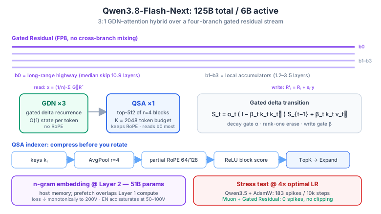
Qwen3.8-Flash-Next is a 125B-total / 6B-active sparse MoE that claims the downstream quality of the previous 397B-A17B flagship (Qwen3.7-Plus) while training on 1/3 the active parameters, 1/3 the tokens, and roughly 1/9 the FLOPs. That is not a tokenizer trick or a benchmark artifact — it is four independent architectural bets stacked on top of each other:
- A 3:1 layer-wise hybrid of Gated DeltaNet (GDN) and (sparse) global attention.
- Qwen Sparse Attention (QSA) with a compressed lightweight indexer, installed during continued pre-training.
- Gated Residual (GR) — a four-branch residual stream with elementwise read gates and data-dependent write gates.
- A 51B-parameter $n$-gram embedding table living off-accelerator in host memory.
Plus a Muon-based optimizer recipe stable enough to survive a $4\times$-overshoot learning-rate stress test with zero loss spikes. This note walks the math of each piece and the empirical evidence behind it.
1. The Blueprint
| Qwen3.8-Flash-Next | Qwen3.7-Plus (predecessor) | |
|---|---|---|
| Total parameters | 125B | 397B |
| Activated per token | 6B | 17B |
| Off-accelerator params | 51B ($n$-gram tables, host memory) | — |
| Training tokens | $1/3$ | $1\times$ |
| Training FLOPs | $\approx 1/9$ | $1\times$ |
The $1/9$ FLOP figure is the headline, and it comes from multiplying two independent $1/3$s: a third of the active capacity times a third of the token budget. Everything else in the report exists to make that product not lose quality — this is the same “shift the Pareto frontier, don’t climb it” framing as SWE-1.7 and MiniMax-M2, applied at the pre-training level rather than the post-training level.
2. Token Mixing: The GDN–Attention 3:1 Hybrid
The bottleneck in scaling long context is the pair of quadratic compute and linear KV growth in softmax attention. Qwen3.8-Flash-Next handles it with a layer-wise schedule: three Gated DeltaNet layers, then one attention layer, repeated.
Block Structure (Repeated):
┌───────────┐     ┌───────────┐     ┌───────────┐     ┌───────────┐
│ GDN Layer │ ──> │ GDN Layer │ ──> │ GDN Layer │ ──> │ QSA Layer │
└───────────┘     └───────────┘     └───────────┘     └───────────┘
The recurrent layers compress context into a fixed-size state at linear cost; the one global attention layer per block retains exact token-level retrieval. This is the same structural bet as Nemotron 3 Ultra and LongCat Flash, but with a delta-rule recurrence rather than Mamba2-style SSM state.
2.1 Gated DeltaNet
Linear attention is best read as a fast-weight memory: a matrix state holding key→value associations. For each head, with query $q_t \in \mathbb{R}^{d_k}$, key $k_t \in \mathbb{R}^{d_k}$, value $v_t \in \mathbb{R}^{d_v}$, GDN carries a state $S_t \in \mathbb{R}^{d_k \times d_v}$ (transposed convention, for implementation efficiency) and runs the gated delta recurrence:
\(\tilde{S}_{t-1} = \alpha_t S_{t-1}\) \(e_t = v_t - \tilde{S}_{t-1}^\top k_t\) \(S_t = \tilde{S}_{t-1} + \beta_t k_t e_t^\top\) \(y_t = S_t^\top q_t\)
where $\alpha_t \in (0,1)$ is a data-dependent decay gate governing state lifetime, $\beta_t \in (0,1)$ is a data-dependent write gate governing update strength, and $e_t$ is the residual error between the value we want to store and the value the current key already retrieves.
The equivalent transition matrix
Substituting $e_t$ back into the update and collecting terms:
\(S_t = \alpha_t S_{t-1} + \beta_t k_t (v_t - \alpha_t S_{t-1}^\top k_t)^\top\) \(S_t = \alpha_t S_{t-1} + \beta_t k_t (v_t^\top - \alpha_t k_t^\top S_{t-1})\) \(S_t = \alpha_t S_{t-1} + \beta_t k_t v_t^\top - \alpha_t \beta_t k_t k_t^\top S_{t-1}\) \(\boxed{S_t = \alpha_t \left( I - \beta_t k_t k_t^\top \right) S_{t-1} + \beta_t k_t v_t^\top}\)
The transition is a decayed rank-one-corrected identity. That form is the whole point.
Why the delta rule matters: targeted erase-and-write
Plain linear attention only adds outer products $\beta_t k_t v_t^\top$, so repeated keys accumulate stale associations without bound. The extra $-\alpha_t \beta_t k_t k_t^\top S_{t-1}$ term is matrix-level house-cleaning: if $k_t$ has been written before, the model retrieves what’s already there, computes the residual $e_t$, and writes only the missing part. Same mechanism as Kimi Delta Attention, which is what makes fast KDA kernels a bellwether workload (see the Cake note).
Feature parameterization
Given normalized input $x_t \in \mathbb{R}^d$, projections pass through causal short 1D convolutions to inject local inductive bias before recurrent compression:
\(q_t = \text{L2Norm}\left(\text{SiLU}\left(\text{ShortConv}(W_q x_t)\right)\right)\) \(k_t = \text{L2Norm}\left(\text{SiLU}\left(\text{ShortConv}(W_k x_t)\right)\right)\) \(v_t = \text{SiLU}\left(\text{ShortConv}(W_v x_t)\right)\)
The L2 normalization on $q_t$ and $k_t$ is load-bearing: it bounds magnitudes so the rank-one delta transition $\left(I - \beta_t k_t k_t^\top\right)$ stays well-conditioned.
Gating dynamics
\(\beta_t = \sigma(W_\beta x_t)\) \(\alpha_t = \exp\left[-\exp(A) \cdot \text{softplus}(W_\alpha x_t + b_\alpha)\right]\)
The double-exponential parameterization keeps $\alpha_t$ in $(0,1)$ with a learnable per-head time constant $A$. Output goes through zero-centered RMSNorm (preventing weight explosion) and a bounded sigmoid output gate rather than SiLU:
\[o_t = W_o \left[ \sigma(W_z x_t) \odot \text{RMSNorm}(y_t) \right]\]The NoPE footnote
Global attention layers keep RoPE. Dropping positional embeddings entirely (a NoPE variant) shows an identical pre-training loss curve — but a severe post-training failure rate in the form of endless generation loops. This is a nice counterpoint to the Kimi K3 architecture derivation, where NoPE does work; the difference is presumably that a 3:1 hybrid has far fewer attention layers to carry positional information, so the remaining ones can’t be asked to infer it implicitly. Loss parity is not architecture parity — a lesson that also shows up in the interplay of training stages.
2.2 Qwen Sparse Attention (QSA)
During continued pre-training at 256K sequence length, the global attention layers are swapped for QSA: queries attend only to a sparse set of token blocks chosen by a lightweight indexer. Architecturally this is the same family as the DSA indexer in DeepSeek-V3.2 and the reuse trick in IndexCache, with a distinctive compression step.
QSA Pipeline:
   Input State (x_i) ──> Projections ──> AvgPool (r=4) ──> Partial RoPE (64/128)
                                                                 │
   Core Attention (Sparse) <── Expand <── TopK Selection <── Block-Causal Score
The compressed lightweight indexer
MQA setup: $H = 4$ query heads, one shared key head.
1. Projections.
\[\hat{q}^h_i = \text{RMSNorm}(W^h_Q x_i), \qquad k_i = W_K x_i\]2. Key compression. Keys are partitioned into non-overlapping blocks of $r = 4$ tokens, average-pooled, and normalized:
\[\hat{k}_b = \text{RMSNorm}\left(\text{AvgPool}(k_{p_b : p_b + r - 1})\right), \quad 0 \le b < \lfloor n/r \rfloor\]with $p_b = b \cdot r$ the block’s starting token index. This is a $4\times$ cut in indexer key state before any scoring happens.
3. Late-stage partial RoPE. RoPE is applied to 64 of 128 dims per indexer head, after pooling:
\[q^h_i = \text{PRoPE}(\hat{q}^h_i, i), \qquad \bar{k}_b = \text{PRoPE}(\hat{k}_b, p_b)\]The ordering is the insight: averaging tokens that already carry different rotary phases would scramble the positional signal into noise. Compress first, rotate second.
4. Block-causal importance scoring. Query $i$ scores block $b$ by head-aggregated, ReLU-activated inner products, under strict block causality:
\[I_{ib} = \begin{cases} \sum_{h=1}^H \text{ReLU}\left(\langle q^h_i, \bar{k}_b \rangle\right), & p_b + r - 1 \le i \\ -\infty, & \text{otherwise} \end{cases}\]ReLU rather than raw dot product means negative-affinity heads abstain instead of voting against, so a single head with strong positive evidence can carry a block into the top-$K$.
5. Top-$K$ and expansion. With token budget $K = 2048$, the block budget is $K_B = \lceil K/r \rceil = 512$. Selected blocks $B_i = \text{TopK}{K_B}({I{ib}}_b)$ map back to token indices, unioned with the tail of the current incomplete block, which is always kept:
\[S_i = \text{Expand}(B_i) \cup \left\{ \left\lfloor \tfrac{i+1}{r} \right\rfloor r, \dots, i \right\}\]Two-stage training protocol
Sparse attention cannot simply be switched on — the backbone was trained against a dense distribution. QSA is installed in two phases:
Stage 1 — dense distillation (1,000 steps, LR $1 \times 10^{-3}$, ~2B tokens). The teacher’s token-level softmax attention $a_{ij}$ is aggregated to block-level targets with MaxPool (preserving salient sparse peaks, which AvgPool would wash out), then L1-normalized:
\[\bar{a}_{ib} = \text{MaxPool}(a_i, p_b : p_b + r - 1), \qquad \hat{a}_i = \frac{\bar{a}_i}{\|\bar{a}_i\|_1}\]The indexer alone is optimized to match:
\[L_{KL} = \frac{1}{N} \sum_i D_{KL} \left( \hat{a}_{i,:} \;\parallel\; \text{Softmax}(I_{i,:}) \right)\]Stage 2 — sparse joint training (8,000 steps, LR $2.5 \times 10^{-5}$, ~200B tokens). Backbone and indexer train together; the backbone adapts to the sparsity pattern $S_i$. The indexer’s KL is now computed only over the selected blocks $B_i$, with teacher targets renormalized inside $B_i$:
\[L_{KL} = \frac{1}{N} \sum_i D_{KL} \left( \hat{a}_{i, B_i} \;\parallel\; \text{Softmax}(I_{i, B_i}) \right)\]Restricting the loss to $B_i$ in stage 2 stops the indexer from spending capacity ranking blocks it will never select — the objective matches deployment.
3. Gated Residual: Widening the Stream
Pre-norm transformers all read and write one residual vector. Every block competes for the same $d$ dimensions of bandwidth, and deep networks pay for it in signal attenuation. Gated Residual (GR) widens the stream to $n_r = 4$ branches, $R \in \mathbb{R}^{n_r \times d}$, read and written through an elementwise gated bottleneck.
Gated Residual (GR) Block Loop:
   Residual Branches R (4 x d) ──> Group RMSNorm ──> Low-Rank Bottleneck (r = d/8) ──> Sigmoid Gate G
                                                                                          │
   R' (Written back) <── Gated Write (s) <── Sublayer Block F(x) <── Elementwise Read (x = G ⊙ R)
This is the same design space as Manifold-Constrained Hyper-Connections, Residual Matrix Transformers, and Attention Residuals — but with a deliberate simplification, discussed below.
3.1 Formulation
Group RMSNorm read. Each branch normalized independently with its own gain $\gamma_i \in \mathbb{R}^d$:
\[\hat{R}_i = \text{RMSNorm}(R_i; \gamma_i), \quad i \in \{1, \dots, n_r\}\]Elementwise dynamic read gating. Gate scores $G \in \mathbb{R}^{n_r \times d}$ come from all branches jointly, through a low-rank bottleneck of rank $r = d/8$:
\[G = \text{unvec}\left( \sigma\left( W_u \,\text{SiLU}\left( \tfrac{1}{n_r} W_d \,\text{vec}(\hat{R}) \right) \right) \right)\]with $W_d \in \mathbb{R}^{r \times n_r d}$, $W_u \in \mathbb{R}^{n_r d \times r}$. The sublayer input is the gated average:
\[x = \frac{1}{n_r} \sum_{i=1}^{n_r} G_i \odot \hat{R}_i\]Data-dependent write gating. The block output $y = F(x)$ is written back with scalar per-branch gates:
\[s = 2 \sigma\left( \tfrac{1}{n_r} W_w \,\text{vec}(\hat{R}) \right), \qquad R'_i = R_i + s_i y\]with $W_w \in \mathbb{R}^{n_r \times n_r d}$. The factor of 2 centers the gate at 1 at initialization, so GR starts as a plain 4-way-replicated residual stream.
3.2 What Do the Branches Actually Learn?
Because GR has no cross-branch mixing, each branch is a plain accumulator — which makes the layer-to-layer information flow exactly traceable. The contribution of block $u$ to block $v$’s input is:
\[a_{u \to v} = \frac{1}{n_r} \sum_{c=1}^{n_r} \frac{G^{(v)}_c \odot \gamma_c \odot s^{(u)}_c y^{(u)}}{\text{rms}\left(R^{(v)}_c\right)}\]reading as: what block $u$ wrote onto branch $c$ ($s^{(u)}_c y^{(u)}$), divided by the scale of branch $c$ at read time, weighted by how much of branch $c$ block $v$ chooses to read ($G^{(v)}_c \odot \gamma_c$).
Comparing against a single-stream reference, $\Delta_{uv} = \pi^{GR}{uv} - \pi^{ref}{uv}$, a clean division of labor emerges:
- Branch 0 is a long-range highway. It is written heavily at Layer 0 (specifically the Layer-0 GDN) and barely touched afterward, so early structural features survive intact across depth — median skip distance 10.9 layers, versus 3.4–3.9 for the others.
- Branches 1–3 are local accumulators, carrying short-range state with median skips of 1.2–3.5 layers.
- Attention layers are the integration hubs. The sublayers that read most heavily from $b_0$ are predominantly the softmax attention layers — global attention is where the model reintegrates the long-range history that the GDN layers compressed away. That is a satisfying mechanistic story for why the 3:1 ratio works: the attention layer isn’t just doing retrieval over tokens, it’s doing retrieval over depth.
3.3 Two Deletions That Paid
- The mixing operator $H_{res}$ was dropped. Designs like Hyper-Connections mix across branches; here that provided no downstream gain while adding large memory read traffic. Without $H_{res}$, the widened stream is traversed exactly once per block in each direction.
- Branches are stored in FP8, halving memory traffic with no measured quality loss — consistent with the low-precision-storage findings in MXFP8 training.
A 4-wide residual stream costs $4\times$ the residual memory traffic if you’re naive about it. These two choices are what make GR affordable rather than merely interesting.
4. The $n$-Gram Embedding Layer
51B parameters of $n$-gram embedding tables sit in host memory, off the accelerator — capacity that costs DRAM, not HBM. This is the same lever as Engram: conditional memory lookup as a way to buy parameters without buying FLOPs or HBM.
- Placement: Layer 2. Shallow enough that a host-memory prefetch, issued as the token enters the network, fully overlaps the compute of Layer 1 — retrieval latency lands off the critical path.
- Vocabulary scaling. Scaling the $n$-gram vocabulary from the base tokenizer size $V = 250\text{K}$ up to $200V$ decreases pre-training LM loss monotonically.
- The downstream disconnect. Loss keeps falling, but downstream English benchmark accuracy saturates or fluctuates past $50V$–$100V$. On Chinese benchmarks (C-Eval, CMMLU), accuracy keeps improving roughly linearly with vocabulary size.
That gap is the most interesting single result in the report. Monotone loss with flat accuracy means the extra $n$-gram capacity is buying probability mass on things the benchmarks don’t test — plausibly surface-form memorization of long-tail multi-byte sequences, which is exactly where a Chinese tokenizer leaves the most on the table. It is another instance of the perplexity-is-the-wrong-metric problem, and a reason to be careful reading loss curves as capability curves (see also metrics across training stages).
5. Optimization and Stability
5.1 Muon, Everywhere 2D
The matrix-aware Muon optimizer is applied to every 2D weight that acts as a linear map: attention projections, GDN projections, MLP experts, and the $n$-gram projections. Momentum orthogonalization uses 8 Newton–Schulz iterations on Nesterov momentum ($\mu = 0.95$). Background on why orthogonalized updates behave differently from AdamW is in SOAP, Muon, and Beyond and SOAP.
Three protocol details that matter more than they sound:
-
Shape-independent RMS updates. The orthogonalized direction is scaled by
\[\gamma(A, B) = 0.2 \sqrt{\max(A, B)}\]making update RMS independent of parameter shape — necessary once the same optimizer touches square attention projections and very rectangular expert matrices.
-
Split fused parameters before orthogonalizing. Fused $qkv$, GDN input projections, and SwiGLU
fc1are split into their independent sub-matrices first. Otherwise orthogonalization mixes singular directions across semantically unrelated operators, and $\gamma(A,B)$ is computed from a fictitious shape. -
Canzona + CUDA Graphs. Megatron-LM shards weights across TP and DP ranks, so Newton–Schulz becomes a load-imbalanced bottleneck. Canzona decouples logical assignment from physical layout, statically reassigning parameters to balance orthogonalization FLOPs across ranks. Splitting fused parameters produces hundreds of small sub-matrix ops, so the whole thing is captured as a CUDA Graph to erase launch overhead — the same pattern as the megakernel arguments in Mixture-of-Kittens.
5.2 Batch-Size Warmup Is Unnecessary — and Harmful
Conventional wisdom ramps batch size to stabilize early training. Scaling sweeps here say the opposite:
- Starting directly at the target $B = 25.2\text{M}$ takes 18.8% fewer optimizer steps than ramping from $6.3\text{M}$ to $25.2\text{M}$ over 524B tokens.
- Warmup runs carry higher gradient noise early (small batches), giving a worse loss up front. Once the target batch is reached, the step-count advantage evaporates under the decay schedule, and the constant-batch baseline finishes with a better final loss.
The mechanism is that batch-size warmup trades wall-clock steps for gradient quality at exactly the phase where the model is most plastic — see Deconstructing Scaling Laws for the general shape of this argument.
5.3 Stress Test: Gating as a Rescaling Mechanism
Under a deliberately brutal test — constant LR held at $4\times$ the optimal value:
| Recipe | Loss spikes / 10k steps | Gradient clipping |
|---|---|---|
| Qwen3.5 architecture + AdamW | 183 | frequently engaged |
| Muon + Gated Residual | 0 | never crossed threshold |
The explanation is the sharpest idea in the report. Without a multiplicative gate, a network pushed by a too-high learning rate has only one way to reduce its effective step: grow activation outliers (observed up to $5000\times$), so that normalization divides everything down. That outlier growth is the instability. GR’s multiplicative gate supplies the rescaling degree of freedom directly, so the network never needs the outliers, and maximum activation levels stay flat. Instability isn’t cured by clipping the symptom; it’s cured by giving the network a cheaper way to do what it was already trying to do. Compare the first-order-approximation view in Stabilizing LLM-RL.
6. Benchmarks
Across fourteen pre-training benchmarks, Qwen3.8-Flash-Next-Base beats the 397B Qwen3.7-Plus-Base on 8 of 14:
| Benchmark | Qwen3.8-Flash-Next-Base (125B / 6B act.) |
Qwen3.8-27B-Base (27B dense) |
Qwen3.7-Plus-Base (397B / 17B act.) |
|---|---|---|---|
| MMLU (5-shot) | 90.36 | 87.51 | 90.43 |
| MMLU-Pro (5-shot, CoT) | 73.23 | 68.60 | 70.90 |
| SuperGPQA (5-shot, CoT) | 51.36 | 44.86 | 48.42 |
| BBH (3-shot, CoT) | 90.87 | 89.56 | 89.41 |
| GSM8K (4-shot, CoT) | 93.29 | 93.18 | 92.95 |
| MATH (4-shot, CoT) | 72.78 | 60.54 | 74.38 |
| EvalPlus (0-shot) | 78.76 | 76.05 | 78.06 |
| MMMLU (5-shot) | 84.86 | 79.74 | 84.53 |
The losses are informative: MMLU is a statistical tie, and MATH is the one clear gap (72.78 vs 74.38). Multi-step symbolic derivation is precisely the workload that benefits from many active parameters and exact long-range attention — the two things a 6B-active 3:1 hybrid economizes on.
7. Takeaways
- Delta-rule linear attention plus one exact attention layer per three is a workable long-context substrate, provided the attention layers keep RoPE. NoPE’s loss-curve equivalence is a trap.
- Compress before you rotate. QSA’s late-stage partial RoPE is a one-line ordering decision worth a $4\times$ indexer-state reduction at no accuracy cost.
- A wide residual stream works best when you don’t mix it. No cross-branch operator means the flow stays analyzable, the memory traffic stays bounded, and the branches spontaneously specialize into one long-range highway plus three local accumulators.
- Multiplicative gating is a stability primitive, not a capacity primitive. Zero loss spikes at $4\times$ LR is a stronger claim than any benchmark row in this report.
- Loss is not accuracy. The $n$-gram vocabulary result — monotone loss improvement, saturating English accuracy, still-climbing Chinese accuracy — should be pinned above the desk of anyone tuning a scaling sweep.
The broader pattern, shared with GLM-5.3-Flash published a day later: the 2026 frontier is not being won by bigger models. It is being won by co-designing architecture, optimizer, and serving stack so that the same quality costs a third of the FLOPs.