Deconstructing Scaling Laws: Optimization, Architecture, and Data
Reading notes on:
- Jianlin Su (2026), 解构Scaling Law:优化、架构、数据的三重奏
Scaling laws are usually presented as a single empirical power law fit to a cloud of runs. Jianlin Su’s framing is sharper: treat the training of a large model as a functional minimization problem, then decompose the loss into layered intervals so each source of error scales independently. This is the theoretical companion to the historical survey in The Architecture of Scaling Laws — where that note traces Kaplan → Chinchilla as a measurement story, this one derives those exponents from a single decomposition and a single inequality.
1. The Core Paradigm: A Triple Decomposition of Loss
Let a model’s performance be $L(\mathcal{E}\mid\mathcal{D},\mathcal{A},\mathcal{O})$ — the error on an ideal distribution $\mathcal{E}$ given a finite dataset $\mathcal{D}$, an architecture $\mathcal{A}$, and an optimizer $\mathcal{O}$. The total distance from a practically-trained state to the theoretical task limit partitions into three additive intervals plus an irreducible floor:
\[\begin{aligned} L(\mathcal{E}\mid\mathcal{D},\mathcal{A},\mathcal{O}) &= \underbrace{L(\mathcal{E}\mid\mathcal{D},\mathcal{A},\mathcal{O}) - L(\mathcal{D}\mid\mathcal{A},\mathcal{O})}_{F_{\text{data}}} \\ &+ \underbrace{L(\mathcal{D}\mid\mathcal{A},\mathcal{O}) - L(\mathcal{D}\mid\mathcal{A},\infty)}_{F_{\text{opt}}} \\ &+ \underbrace{L(\mathcal{D}\mid\mathcal{A},\infty) - L(\mathcal{D}\mid\infty,\infty)}_{F_{\text{arch}}} \\ &+ L(\mathcal{D}\mid\infty,\infty). \end{aligned}\]Each interval isolates one bottleneck:
- Data error $F_{\text{data}}$ — the generalization gap, the penalty for training on a finite sample $\mathcal{D}$ instead of the true distribution $\mathcal{E}$.
- Optimization error $F_{\text{opt}}$ — the gap to a “perfect optimizer” ($\infty$ steps, ideal hyperparameters); it isolates learning rate $\eta$, batch size $B$, and step count $T$.
- Architecture error $F_{\text{arch}}$ — the inherent expressive limit of the model structure (parameters $N$, width $W$, depth $H$) relative to an infinitely expressive hypothesis class.
Establishing these layered minima is the prerequisite for predicting behavior across orders of magnitude — you optimize each term against its own scale variable.
2. The Engine: An Inequality of Heterogeneous Powers
Scaling laws are power laws because of scale invariance: $f(\lambda x) = \lambda^{-\gamma} f(x)$. Almost every optimal-allocation result below reduces to minimizing $ax^p + bx^{-q}$ — one term that grows with $x$, one that shrinks. The weighted AM-GM inequality $\sum w_i x_i \ge (\sum w_i)\prod x_i^{w_i/\sum w_i}$ handles it in one stroke. Assigning weights $w_1 = q$, $w_2 = p$:
\[ax^p + bx^{-q} = q \cdot \frac{ax^p}{q} + p \cdot \frac{bx^{-q}}{p} \ge (p+q)\left(\frac{a^q b^p}{p^p q^q}\right)^{\frac{1}{p+q}},\]with equality — the optimum — when the weighted terms balance, giving the closed form
\[x^\star = \left(\frac{bq}{ap}\right)^{\frac{1}{p+q}}.\]Under a sum constraint (minimize $ax^{-p} + by^{-q}$ subject to $x+y=1$, as in width-vs-depth allocation) there is no elementary closed form, but the Lagrangian gives $\frac{x^{p+1}}{(1-x)^{q+1}} = \frac{ap}{bq}$. The left side is monotone on $(0,1)$, so a unique root exists by the intermediate value theorem — solve by bisection. This single lemma is the workhorse for everything that follows.
3. Optimization Scaling Laws: Learning Rate and Batch Size
Model $F_{\text{opt}}$ as a tension between progress (effective distance $T\eta$) and stochastic noise (governed by $B$ and $\eta$):
\[F_{\text{opt}} \sim \alpha_1 (T\eta)^{-\gamma_1} + \alpha_2 B^{-\gamma_2} + \alpha_3 \eta^{\gamma_3}.\]Theoretical analyses of SignSGD and Muon suggest critical exponents $\gamma_1 = 1$, $\gamma_3 = 1$, $\gamma_2 = \tfrac12$.
Optimal learning rate. Applying the heterogeneous-power lemma to $\eta$:
\[\eta^\star \sim \left(\frac{\alpha_1 \gamma_1 T^{-\gamma_1}}{\alpha_3 \gamma_3}\right)^{\frac{1}{\gamma_1+\gamma_3}} \sim T^{-\frac{\gamma_1}{\gamma_1+\gamma_3}}.\]This exposes a real tension in the empirical literature: Microsoft Law finds $\eta^\star$ negatively correlated with total samples $K$, while Step Law posits more complex dependencies. Under theoretical values $\gamma_1 = \gamma_3 = 1$ we get $\eta^\star \sim T^{-1/2}$, which becomes $\eta^\star \sim K^{-1/4}$ once $B^\star$ is folded in — remarkably close to Microsoft Law’s measured $K^{-0.32}$.
Optimal batch size. Fix total samples $K = BT$, assume optimal $\eta$, and the law simplifies to $\tilde\alpha_1 T^{-\tilde\gamma_1} + \alpha_2 B^{-\gamma_2}$. Minimizing over $B$:
\[B^\star \sim K^{\frac{\tilde\gamma_1}{\tilde\gamma_1 + \gamma_2}}.\]With $\tilde\gamma_1 = \gamma_2 = \tfrac12$, this gives $B^\star \sim K^{1/2}$ — consistent with Step Law’s $K^{0.571}$.
Why $B^\star$ is $N$-independent. Kaplan and Chinchilla both observe that optimal batch size barely moves with model size $N$. Treating the coefficients as functions of $N$ ($\alpha_1 N^{-\gamma_5}$, $\alpha_3 N^{\gamma_7}$, …), $N$-independence of $B^\star$ and $F_{\text{opt}}^\star$ requires exactly $\gamma_3\gamma_5 = \gamma_1\gamma_7$ and $\gamma_6 = 0$. Optimization efficiency stays stable as capacity scales precisely when these coupling constraints hold.
4. Architectural Scaling Laws: Width, Depth, Sparsity, Memory
Stop treating $N$ as a monolithic scalar. Split it into width $W$ and depth $H$ with $N \sim W^2 H$, and model $F_{\text{arch}} \sim \alpha_W W^{-\gamma_W} + \alpha_H H^{-\gamma_H}$. Substituting $H \sim N W^{-2}$:
\[F_{\text{arch}} \sim \alpha_W W^{-\gamma_W} + \alpha_H N^{-\gamma_H} W^{2\gamma_H}.\]With theoretical $\gamma_W = \gamma_H = 1$, the optimum is
\[W^\star \sim N^{1/3}, \qquad H^\star = N/(W^\star)^2 \sim N^{1/3}.\]Optimal scaling grows width and depth in equal $1/3$-power proportions — a clean, falsifiable prescription.
Compute-optimal (Chinchilla). Under fixed compute $C \sim NK$, minimize $F_{\text{opt}}^\star + F_{\text{arch}} \sim \hat\alpha_1 K^{-\hat\gamma_1} + \alpha_4 N^{-\gamma_4}$:
\[N^\star \sim C^{\frac{\hat\gamma_1}{\hat\gamma_1+\gamma_4}}, \qquad K^\star \sim C^{\frac{\gamma_4}{\hat\gamma_1+\gamma_4}}.\]With $\hat\gamma_1 = \tfrac14$ and $\gamma_4 = \tfrac13$ this yields $N^\star \sim C^{3/7}$ and $K^\star \sim C^{4/7}$ — parameters and data scale nearly in tandem, recovering the Chinchilla observation from first principles rather than from a curve fit.
Sparsity (MoE). Map a Mixture-of-Experts model to a dense equivalent via an effective parameter count:
\[N_{\text{eff}} = N_{\text{act}}^{\frac{\gamma_{\text{act}}}{\gamma_{\text{act}}+\gamma_{\text{total}}}}\, N_{\text{total}}^{\frac{\gamma_{\text{total}}}{\gamma_{\text{act}}+\gamma_{\text{total}}}}.\]To forbid the degenerate $N_{\text{act}} \to 0$, add an “efficiency-lever” penalty $\alpha_8 N_{\text{act}}^{-\gamma_8}$ that keeps a functioning representation. This is the theory under the extreme-sparsity designs like Kimi K3’s 896-choose-16 routing and the milder ratios in GLM-5.2 and Inkling.
Heterogeneous memory. Combining MoE with memory layers (PKM, Engram) obeys the identity $N_{\text{moe}} + N_{\text{mem}} = N_{\text{total}} + N_{\text{act}}$. Treating the right side as a fixed budget, the sum-constraint optimizer from §2 pins down the unique optimal split between computation-heavy experts and retrieval-heavy memory.
5. Data Scaling and Multi-Epoch Training
$F_{\text{data}}$ is the finite-data penalty, dominated by the multi-epoch overfitting cost of repetition $K/D$:
\[F_{\text{data}} \sim \alpha_9 D^{-\gamma_9} + \alpha_{10}\,(K/D)^{\gamma_{10}},\]or the more flexible $\alpha_{10} K^{\gamma_{10}} D^{-\gamma_{11}}$ for epoch-scaling predictions across regimes. Balancing the optimization gain $K^{-\hat\gamma_1}$ against the repetition penalty:
\[K^\star \sim D^{\frac{\gamma_{10}}{\hat\gamma_1 + \gamma_{10}}}.\]As $D$ grows, the optimal epoch count $K^\star/D$ decreases: massive datasets are best consumed single-pass, while data-constrained regimes need multiple passes to reach the $F_{\text{opt}}$ floor — but never without an overfitting cost. This is the same wall analyzed empirically in The Architecture of Scaling Laws; data scaling stays “blurry” mostly because quality and domain distribution resist a stable scalar parameterization.
6. The Kaplan–Chinchilla Divergence, Quantified
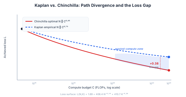
Where this decomposition pays off is in explaining cost. Kaplan’s parameter-heavy rule ($N \propto C^{0.73}$) diverges rapidly from Chinchilla’s compute-optimal path ($N \propto C^{0.45}$): parameter count balloons at the expense of tokens, and evaluating both allocations against the same Chinchilla loss surface $L(N,K) = 1.69 + 406.4\,N^{-0.34} + 410.7\,K^{-0.28}$ shows the gap widening with scale — reaching a +0.38 loss gap at $10^{24}$ FLOPs.
7. Why Power Laws? Coefficients vs. Exponents
The dominance of power laws reflects the physics of scale-invariant systems. Unlike exponential (“short-tail”) decay — where a resource quickly hits zero marginal utility — the long-tail power law permits continuous improvement across infinite scales, because the fundamental difficulty of the task stays constant regardless of the model’s absolute size.
This motivates a clean engineering/nature duality:
- Exponents ($\gamma$) are the critical exponents of the problem — the natural difficulty of the distribution $\mathcal{E}$ and the task. They are rarely moved by engineering.
- Coefficients ($\alpha$) are the engineering lever. Better optimizers, residual connections (e.g. AttnRes), or hardware efficiency reduce $\alpha$ within a specific decomposition layer — a better optimizer shrinks the $\alpha$ of $F_{\text{opt}}$, not its exponent.
Takeaway. Escaping the “alchemy” of large-scale training is a matter of dimensional analysis. Treat hyperparameters not as isolated toggles but as scale-invariant units inside a triple-decomposed loss, and each of Chinchilla’s $C^{3/7}$, Step Law’s $B \sim K^{0.57}$, and the $N^{1/3}$ width–depth rule falls out of one inequality applied to the right interval. That is the transition from heuristic experimentation to the rigorous derivation of optimal intelligence — and it feeds directly into the joint pretraining-to-RL scaling law, where the pretraining loss $L_{pt}$ these laws govern becomes the input to downstream RL.