From Pretraining to RL: A Joint Scaling Law for Reasoning
Reading notes on:
The modern LLM pipeline is large-scale pretraining, then post-training (SFT and RL). We have solid scaling laws for pretraining (Chinchilla) and, increasingly, for RL in isolation — see Predictable Scaling of Reinforcement Learning for LLMs. What’s been missing is the interface: how a pretrained model’s properties (size $N$, data $T$, loss $L_{pt}$) quantitatively determine its responsiveness to RL compute. This paper closes that gap with a single joint scaling law — and does it in a controlled testbed where the ground truth is verifiable.
1. The Testbed: Chess as a Controlled LLM Proxy
Frontier LLMs are the wrong place to study this — compute is prohibitive and the datasets are uncontrolled. Instead the authors mirror the full LLM pipeline in chess:
- Pretrain autoregressive models (5M → 1B params) on human chess games.
- SFT on synthetic Chain-of-Thought reasoning traces.
- RL with Group Relative Policy Optimization (GRPO) and verifiable binary rewards (did the move win?).
Chess gives cheap, unambiguous verifiers and full control over data — the same appeal that makes RLVR-style setups attractive for studying reasoning limits.
2. Standardizing Compute Across Stages
To compare stages you need a common currency. The authors use the standard dense estimate $C_{train}(N, T) \approx 6NT$:
- Pretraining: $C_{pt} = 6NT_{pt}$.
- SFT: $C_{sft} = 6 N E_{sft} n_{sft} L_{sft}$ (scales with epochs and context length).
- RL (GRPO): rollout generation, reference-model evaluation, and policy optimization take multiple passes, estimated as $C_{rl} = 10 N T_{rollout}$.
3. Deriving the Joint Scaling Law
Pretraining: the Chinchilla form
Fit the classic form to the pretraining sweep:
\[L_{pt}(N, D) = E + \frac{A}{N^\alpha} + \frac{B}{D^\beta}.\]For chess they find $\alpha \approx 0.40$ and $\beta \approx 0.68$ — validation loss falls substantially faster with tokens than with parameters relative to natural-language modeling. (For the functional-form background, see The Architecture of Scaling Laws.)
RL: from sigmoid to log-linear
Prior work models a fixed model’s performance under RL compute as a sigmoid:
\[R_{sig}(C) - R_0 = (A - R_0)\,\frac{1}{1 + (C_{mid}/C)^\gamma}.\]But running RL to saturation to find the asymptote $A$ for every configuration is impossibly expensive. So the authors take a first-order Taylor expansion of the sigmoid around a reference compute level $x_{ref} = \log_{10} C_{ref}$, in the non-saturated regime:
\[R_{sig}(x) \approx R_{sig}(x_{ref}) + \frac{dR_{sig}}{dx}\Big|_{x=x_{ref}}(x - x_{ref}).\]This linearizes the local trajectory into a log-linear law:
\[R_{N,T}(C) = R^{ref}_{N,T} + B_{N,T}\,(\log_{10} C - \log_{10} C_{ref}).\]Differentiating the sigmoid gives the theoretical local slope:
\[B_{N,T} \approx \gamma \ln(10)\,\frac{R^{ref}_{N,T} - R_0}{A - R_0}\,(A - R^{ref}_{N,T}).\]This first-order-around-a-reference trick is the same spirit as the linearization in First-Order Approximation for Stable LLM-RL Training.
The bridge
Now express both the reference reward and the slope purely in terms of pretraining variables:
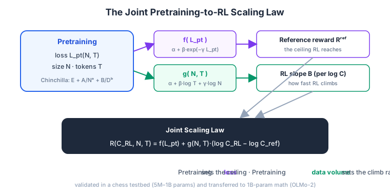
- Reference reward — post-RL performance is remarkably predictable from pretraining eval loss alone, via an exponential map: $f(L_{pt}) = \alpha_f + \beta_f \exp(-\gamma_f L_{pt})$.
- RL slope — how fast RL improves is driven mainly by pretraining data volume, not just model size: $g(N, T) = \alpha_g + \beta_g \log_{10} T + \gamma_g \log_{10} N$.
Combining yields the Joint Pretraining-RL Scaling Law:
\[R(C_{RL}, N, T) = f(L_{pt}(N, T)) + g(N, T)\,(\log_{10} C_{RL} - \log_{10} C_{ref}).\]In words: pretraining loss sets the ceiling RL can reach quickly; pretraining data volume sets the climb rate.
4. Where Should the FLOPs Go?
Tracing the compute-optimal frontier from the joint law:
- RL is initialization-limited. At low total compute, starting RL on a weakly pretrained model wastes it — keep the bulk in pretraining.
- The optimal RL fraction grows with scale. As total compute rises and initialization is strong enough, the RL share increases: from ~20% at 50M params to ~28% at 680M params.
- Pass@1 vs. pass@k. Pretraining scale is the dominant driver of large-$k$ pass@k (broad coverage of good solutions), while RL directly optimizes pass@1.
5. What Does RL Actually Do?
The perennial debate: does RL merely sharpen existing capabilities, or discover new ones? Analyzing per-move probability distributions before/after RL, the authors find RL is not uniform temperature scaling. It redistributes mass differently by difficulty:
- Easy puzzles — ground-truth amplification. RL mostly boosts correct moves the SFT policy already ranked top-k.
- Hard puzzles — tail discovery and wrong-mode amplification. RL surfaces correct moves from the deep tail (initially $<0.05$ probability) into the top-k — but simultaneously over-reinforces incorrect moves that SFT mistakenly favored.
This mixed redistribution is exactly why RL reliably boosts pass@1 but often fails to improve pass@k — echoing the ceiling observed in Reasoning Limits of LLMs Under RLVR. Parsing the CoT trees adds a second mechanism: during RL, models expand search breadth (branching factor) rather than depth — better candidate generation and selection, but still unable to recover continuations deeper than ~5 moves.
6. Transfer to Math
To show these are not chess artifacts, the authors pretrain a 1B natural-language model (OLMo-2 architecture) on up to 200B tokens of math and RL-tune with GRPO on GSM8K/MATH. The same patterns hold:
- Post-RL reference performance is predicted well by intermediate pretraining loss.
- The RL reward slope improves linearly with $\log_{10}$ pretraining tokens.
Takeaway
Pretraining and post-training are deeply coupled, and the coupling is quantitative: $L_{pt}$ fixes the reachable ceiling, and pretraining data volume fixes the RL climb rate. This complements the distributional view of what each stage does in The Distributional Lens of Post-Training, and it reframes the reasoning-effort question from The Mechanics of Reasoning Effort and Inference Scaling as an allocation problem across the whole pipeline. The next frontier is clear from the mechanistic story: taming wrong-mode amplification on hard tasks is what stands between “better pass@1” and genuinely deeper reasoning. And of course, none of this happens without the pretraining optimizer that sets $L_{pt}$ in the first place — the subject of SOAP, Muon, and Beyond.