Kimi K3: Open Frontier Intelligence at 2.8 Trillion Parameters
Reading notes on:
- Kimi K3: Open Frontier Intelligence (announcement blog)
- Kimi K3 Technical Report (architecture & infra deep dive)
1. Executive Summary
Kimi K3 is a 2.8-trillion-parameter (3T-class) Mixture-of-Experts model with 104B activated parameters, a native 1M-token context window, and native vision. While it trails proprietary models like Claude Fable 5 and GPT-5.6 Sol, it sets a new upper bound for open weights and shows a 2.5× improvement in scaling efficiency over Kimi K2 (see the Kimi-K2 Reading Note). The gains come from co-designing the architecture, the training recipe, and the serving infrastructure — the same open-frontier lineage as LongCat-2.0, GLM-5.2, and Inkling.
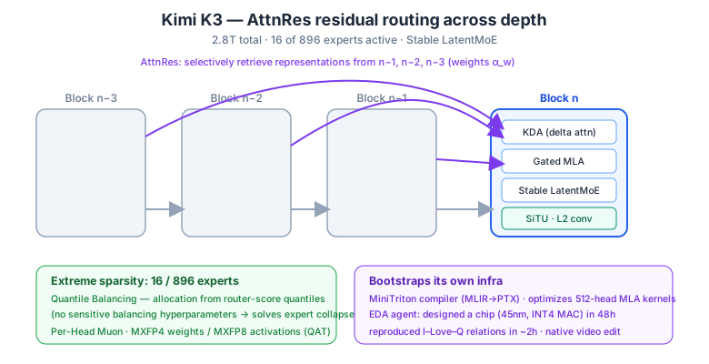
The rest of these notes deconstruct the math and systems that make this scale trainable and servable: the hybrid attention stack, the depth-wise information routing, the extreme-sparsity stabilizers, the perfectly load-balanced expert-parallel plan, and the deployment-aware post-training and serving pipeline. For a first-principles derivation of why the key design choices work — the $\mathcal{O}(|x|^4)$ SiTU-GLU outlier, the single RMS Norm, and the DeltaNet↔RoPE equivalence behind NoPE — see the companion Kimi K3 Architecture, Derived.
2. Hybrid Attention: KDA + Gated MLA
K3 abandons pure global attention for a layerwise hybrid structure: 3 Kimi Delta Attention (KDA) layers for every 1 Gated Multi-head Latent Attention (MLA) layer. The Gated MLA layers handle global content interaction without positional encodings (NoPE); the KDA layers carry position-sensitive, recency-aware sequence mixing. This builds directly on the Linear Attention: Kimi Delta Attention line of work.
KDA extends the delta-rule recurrence with a channel-wise forget gate. For query $q_t$, key $k_t$, value $v_t$, and recurrent state $S_t$:
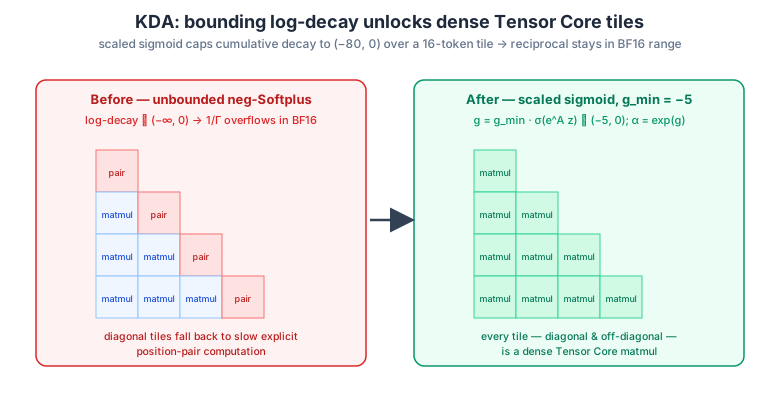
\[S_t = \left( I - \beta_t k_t k_t^\top \right) \text{Diag}(\alpha_t) S_{t-1} + \beta_t k_t v_t^\top, \qquad \tilde{o}_t = S_t^\top q_t.\]Solving the intra-chunk bottleneck. In chunkwise-parallel execution, KDA rescales keys by the reciprocal cumulative decay $1/\Gamma_{1 \to C}^{[t]}$. Previous implementations (like Kimi Linear) mapped decay logits to log-decay with an unbounded negative-Softplus, which could overflow in BF16 and forced diagonal blocks onto slow, explicit position-pair computation. K3 replaces this with a scaled sigmoid that bounds the log-decay:
\[g_t^h = g_{\min}\,\text{Sigmoid}\!\left(e^{A^h} z_t^h\right) \in (g_{\min}, 0)^{d_k}, \qquad \alpha_t^h = \exp(g_t^h) \in (e^{g_{\min}}, 1)^{d_k}.\]Hard-coding $g_{\min} = -5$ restricts the cumulative log-decay over a 16-token tile to $(-80, 0)$. This finite range keeps the reciprocal inside BF16 dynamic range, so both diagonal and off-diagonal tiles run as dense Tensor Core matmuls — the diagonal position-pair bottleneck disappears entirely.
3. Attention Residuals: Replacing the “RNN of Depth”
Standard residual connections $\sum f(x)$ behave like an RNN over depth, compressing all prior-layer representations into a single bottleneck state. K3 adopts Attention Residuals (AttnRes) — from the Attention Residuals (AttnRes) framework — letting each layer $l$ selectively attend to representations from all preceding layers. With a learned pseudo-query $q_l$:
\[\alpha_{i \to l} = \frac{\exp\!\left(q_l^\top \text{RMSNorm}(k_i)\right)}{\sum_{j=0}^{l-1} \exp\!\left(q_l^\top \text{RMSNorm}(k_j)\right)}.\]Full AttnRes costs $O(Ld)$ memory — too expensive. K3 chunks its 93 layers into 8 blocks, sums outputs within a block into a single block-level representation, and attends only across the $N$ blocks. That drops overhead to $O(Nd)$ while recovering most of the benefit.
4. Stable LatentMoE: SiTU-GLU + Quantile Balancing
K3’s MoE is extremely sparse: 896 routed experts per layer, 16 active per token (~1.7% activation). Contrast the milder 8/256 in GLM-5.2 and the mini-activation approach in MiniMax-M2. At this sparsity, the chain of consecutive matmuls produces exploding activations, so the Stable LatentMoE framework adds two stabilizers.
SiTU-GLU vs. SwiGLU. The industry-standard SwiGLU ($x \cdot \text{Sigmoid}(x) \cdot W_u x$) is unbounded on both the gate and up branches, so coincident large coordinates create massive outliers. K3 introduces the Sigmoid Tanh Unit GLU (SiTU-GLU) with a softcap $\text{softcap}(x, \beta) = \beta \tanh(x/\beta)$:
\[\text{SiTU-GLU}(x) = \left[ \beta_1 \tanh\!\left(\frac{W_g x}{\beta_1}\right) \odot \text{Sigmoid}(W_g x) \right] \odot \left[ \beta_2 \tanh\!\left(\frac{W_u x}{\beta_2}\right) \right].\]With $\beta_1 = 4$ and $\beta_2 = 25$, the output is bounded by $\beta_1 \beta_2 = 100$ — strictly preventing overflow while matching SwiGLU’s approximately linear local response near the origin to first order.
Quantile Balancing (QB). To balance 896 experts without an auxiliary loss, K3 sets an expert-specific bias $b_j$ from the $(1 - k/n)$-quantile of router margins. Computing an exact global quantile across millions of tokens would cost $O(mn)$ communication; instead K3 uses a histogram estimator — bin the margins into a counts matrix and aggregate via a single cheap all-reduce — eliminating residual load imbalance with negligible overhead. (Optimizer side: K3 also extends Muon per attention head; see SOAP, Muon, and Beyond and SOAP.)
5. Infrastructure: Perfect Load Balancing with MoonEP
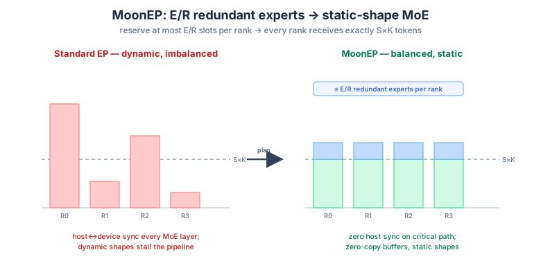
Traditional MoE Expert Parallelism suffers from computational imbalance — token loads fluctuate per expert. K3’s MoonEP proves a clean theorem: a perfectly balanced plan across EP ranks always exists using at most $E/R$ redundant experts, where $E$ is the total number of experts and $R$ is the EP size.
By reserving exactly $E/R$ redundant slots per rank, the planner guarantees a feasible solution where every rank receives exactly $S \times K$ tokens. This turns MoE training from a dynamic-shape process into static-shape execution — no host–device synchronization at every MoE layer, and zero-copy communication buffers. It’s the fully-balanced, zero-host-sync-on-the-critical-path property that expert-parallel systems like MoE Parallel Folding chase.
6. Post-Training: 9-Expert MOPD and Partial Rollouts
Fine-tuning one model to handle diverse agentic tasks across reasoning-effort levels is hard, and long-horizon agentic RL suffers from extreme tail latencies during rollout. K3 scales RL across three domains (general, general agents, coding agents) × three reasoning-effort levels (low, high, max) = 9 specialized expert policies.
Multi-Teacher On-Policy Distillation (MOPD). To consolidate the 9 capabilities back into one model, K3 aligns the student $\pi_\theta$ with the domain-and-effort-specific teacher $\pi_{\text{teacher}}^{(d,e)}$ via a clipped likelihood ratio used as a dense reward:
\[r_{\text{opd}}(y_t) = \text{clip}\!\left(\text{sg}\!\left(\log \frac{\pi_{\text{teacher}}^{(d,e)}(y_t \mid x, y_{<t})}{\pi_\theta(y_t \mid e, x, y_{<t})}\right), -R_{\max}, R_{\max}\right).\]This slots straight into the RL framework — the on-policy distillation discipline covered in Revisiting On-Policy Distillation and the Distributional Lens of Post-Training.
Partial rollouts. Rather than waiting for a full 1M-token trajectory before updating, generation pauses once a fraction $\lambda$ of active trajectories finish. Paused rollouts are enqueued and prioritized for resumption next iteration, while policy updates proceed with localized per-token regularization to absorb the resulting off-policy staleness — the trainer/generator matching problem from RL Systems Mind the Gap.
7. Scaling to 1M Tokens: NoPE and KDA Context Parallelism
Because K3 uses NoPE in its periodic MLA layers and handles position entirely through the KDA decay mechanism, it extrapolates to 1M-token contexts natively — no RoPE rescaling hacks. Context length grows progressively from 8K → 64K during pre-training, and 256K → 1M during cooldown.
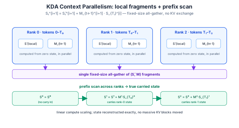
KDA Context Parallelism (KCP). Standard sequence parallelism (ranks exchange KV blocks) is insufficient for KDA, whose delta rule applies a token-dependent transition $M_t = (I - \beta_t k_t k_t^\top)\text{Diag}(\alpha_t)$ to the incoming state before the current write. Because a local segment’s effect depends on the incoming state, it can’t be computed from a zero state. KCP decomposes the recurrent update across $P$ ranks. For a state entering rank $i+1$, after $t$ local tokens:
\[S_t^{[i+1]} = \tilde{S}_t^{[i+1]} + M_{t \leftarrow 1}^{[i+1]} S_{T_i}^{[i]},\]where $M_{t \leftarrow 1}^{[i+1]}$ is the cumulative transition on the incoming state and $\tilde{S}_t^{[i+1]}$ is the locally-generated-from-zero fragment. Each rank exchanges only these two fragments via a single fixed-size all-gather, then reconstructs the true state via a prefix scan across ranks — linear compute scaling with no massive KV exchange. (Compare the balanced-SP approach for another modality in Scaling Video Training with Sequence Parallelism.)
8. Deployment-Aware Post-Training: MXFP4 QAT + EAGLE-3
Serving a 2.8T-parameter MoE demands the inference story be baked into post-training.
- Quantization-aware training. The MoE expert weights (the bulk of the footprint) are quantized to MXFP4 with MXFP8 activations, and QAT runs throughout both SFT and RL so the model natively adapts to precision loss — rollout and training share the exact same quantization scheme. This is the low-precision-in-the-loop discipline from The 4-bitter Lesson: NVFP4 in the RL Loop and Quantization-Aware Distillation (QAD).
- Draft model via LK Loss. K3 is pre-trained with a multi-token-prediction (MTP) layer, fine-tuned into an EAGLE-3-style draft model for speculative decoding. Instead of the usual KL surrogate, the draft directly optimizes the LK Loss — the negative log of the theoretical acceptance rate:
This makes the capacity-limited draft maximize token acceptance at inference time.
9. Serving Infrastructure: KDA-Aware Prefix Caching
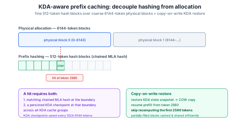
In a hybrid architecture the MLA KV cache grows with sequence length and is paged per token, while the KDA recurrent state is fixed-size per sequence. Standard block-hash prefix caching breaks: KDA checkpoints are expensive and can only be saved sparsely (every 1024–6144 tokens), which would pin prefix matching to those coarse blocks.
K3 decouples hashing granularity from physical block size: prefix hashing runs on fine 512-token hash blocks while physical allocation uses 6144-token blocks. A cache hit requires matching the MLA chained hash and locating a persisted KDA checkpoint at that boundary across all KDA cache groups. A request hitting deep inside a physical block (say token 2560) restores the KDA snapshot, copies it copy-on-write, and resumes prefill without recomputing the first 2560 tokens. This custom prefill cache was contributed to vLLM, and serving is optimized for supernodes of 64+ accelerators.
10. Multimodal Training and the AgentENV Sandbox
Scrapping contrastive pre-training. Prior models (like Kimi K2.5) initialized vision encoders from contrastively pre-trained models (e.g., SigLIP). K3 found this harms stability — attaching SigLIP to the LLM backbone caused frequent gradient spikes during joint optimization. Training MoonViT-V2 entirely from scratch via next-token prediction shapes the representations natively by the language-modeling objective, yielding much smoother gradient norms with no downstream visual degradation.
AgentENV. Container-based sandboxes buckled under agentic RL — kernel panics and deadlocks when the model mounted disks or launched nested containers. K3’s RL environments use AgentENV, built on Firecracker microVMs, giving high-fidelity isolation plus incremental checkpointing with resume latencies as low as 49 ms. Since models spend up to 98% of sandbox lifetime waiting on inference, AgentENV pauses idle sandboxes (zero CPU/memory), forks them for reward judging without side effects, and uses copy-on-write memory to hit a 6.5× memory overcommit across thousands of concurrent environments — the terminal-agent-at-scale regime explored in ECHO.
11. Capabilities
K3’s agentic strength shows on domain tasks rather than static benchmarks:
- GPU compiler development: autonomously built MiniTriton — a tile-level IR over MLIR, optimization passes, and a PTX codegen pipeline — rivaling or beating Triton on some workloads and sustaining stable nanoGPT training.
- Kernel optimization: optimized 512-head-dim MLA, KDA, and AttnRes kernels on H200 and alternative GPGPUs, outperforming GPT-5.6 Sol and Claude Opus 4.8 — the model-writes-its-own-kernels frontier that abstractions like CODA are built to enable.
- Autonomous chip design: as an EDA agent, designed a nano-model chip on Nangate 45nm in 48 hours — 4 mm², timing closed at 100 MHz, 8,700 tokens/s decode, 1.46M standard cells, 0.277 MB SRAM, an INT4 MAC array with fused dequantization.
- Scientific workflows: reproduced I–Love–Q universal relations in ~2 hours (a 1–2 week human task), synthesizing 20+ papers, 300+ equations of state, and 3,000+ lines of Python.
- Multimodality: native text/image/video; multi-agent setups (20+ subagents over 391 gravitational-wave events) and autonomous video editing (motion-matched cuts, beat sync from 56 clips).
12. Limitations
- Statefulness: K3 is highly sensitive to preserved “thinking history.” Switching models mid-session or using harnesses that drop historical context causes unstable generation — an operational hazard familiar from Harness Engineering for Self-Improvement.
- Excessive proactiveness: trained for long-horizon autonomy, K3 makes unprompted decisions under ambiguity; production use needs explicit constraints via system prompts or
AGENTS.md.
Takeaway: the throughline is bounding the unbounded. A scaled-sigmoid decay bound makes KDA a dense-matmul kernel; SiTU-GLU’s softcap tames extreme-sparsity outliers; Quantile Balancing replaces fragile heuristics with a quantile estimator; and MoonEP’s $E/R$-redundancy theorem converts dynamic MoE shapes into static execution. Combined with QAT-in-the-loop, KDA-aware caching, and microVM sandboxes — plus K3’s ability to bootstrap its own low-level systems (PTX codegen, INT4 MAC arrays, 512-head MLA kernels) — it marks an inflection point where open-weights AI can directly accelerate its own hardware and software lifecycle.