CODA: Optimizing Transformers via GEMM-Epilogue Programming
Reading notes on:
We usually think of LLM training as compute-bound — dominated by massive matrix multiplications. But modern training is increasingly throttled by the memory wall. Non-GEMM operations — normalization, activations, residual updates, reductions — account for a nontrivial fraction of end-to-end GPU time precisely because they are deeply memory-bound: they shuttle large intermediate tensors through global memory while doing very little arithmetic. This is the same bandwidth-bound regime dissected in Efficiency in LLMs: Mastering Fast Inference and Memory Bandwidth and The Economics of a Token.
CODA is a GPU kernel abstraction that attacks this by algebraically reparameterizing Transformer blocks into GEMM-plus-epilogue programs.
1. The Epilogue Concept
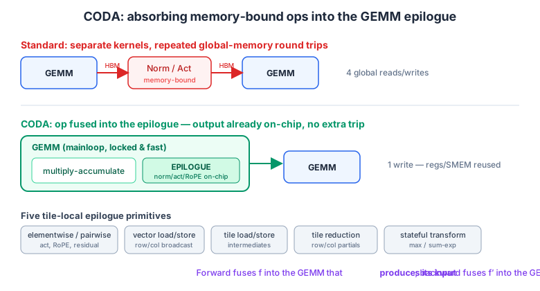
A high-performance GEMM kernel has two parts: the mainloop (the matrix multiply-accumulate) and the epilogue (which transforms the output tile and writes it to global memory). Because the GEMM output already sits in on-chip memory (registers / shared memory), applying operations in the epilogue eliminates additional global-memory round trips. This is the same on-chip-locality principle that Blackwell’s TMEM and TMA hardware push further in NVIDIA Blackwell SM100.
CODA locks down the highly optimized GEMM mainloop and exposes five classes of heavily constrained, tile-local epilogue primitives:
- Elementwise / pairwise maps — activations, RoPE, residuals.
- Vector loads / stores — broadcasting row/column vectors.
- Tile loads / stores — intermediate values.
- Tile reductions — partial reductions over rows/columns.
- Stateful transforms — running tile states such as max / sum-exp for softmax.
2. Forward-Pass Reparameterizations
The trick is to make memory-bound operations fit into a tile-local epilogue via algebraic rewriting.
GEMM → Residual → RMSNorm → GEMM
A standard block runs GEMM → Residual → RMSNorm → GEMM. Normally RMSNorm reduces across the entire hidden dimension (larger than a tile), which blocks fusion. Let $z$ be the residual stream, $\gamma$ the RMSNorm weight, and $r = 1/\text{rms}(xW_0 + z)$ the row-wise inverse RMS factor. The canonical computation is:
Because $r$ is a row-wise scalar shared across the feature dimension, it commutes with the projection $W_1$:
\[y = r\big((xW_0 + z) \odot \gamma\big)W_1\]So the normalization scalar $r$ need not be applied before the second GEMM — it can be delayed into the epilogue of the second GEMM. CODA decomposes this into:
- GEMM 1 + epilogue: compute $h_2[i,j] = (xW_0[i,j] + z[i,j]) \odot \gamma[j]$ and emit a tile-local partial sum-of-squares $\hat{r}[i,j]$.
- Auxiliary kernel: a tiny bandwidth-light reduction over $\hat{r}$ to obtain row-wise $r$.
- GEMM 2 + epilogue: project and apply the delayed scaling $y[i,j] = r[i]\,h_3[i,j]$.
Pairwise activations (SwiGLU, RoPE)
SwiGLU and RoPE are pairwise — they consume two adjacent feature values. Naive implementations materialize the full GEMM output in global memory first. CODA instead matches the output arrangement to the Hopper Tensor Core accumulator layout, where each thread already holds a tuple of adjacent outputs in registers. Applying the pairwise map at the register level in the epilogue avoids materializing the expanded SwiGLU intermediate entirely.
Cross-entropy loss
The per-token loss is $\ell_i = -h_{i,y_i} + \log \sum_k \exp(h_{i,k})$. CODA fetches the target logit via an indexed load in the epilogue while accumulating log-sum-exp as tile-local max and sum-exp statistics; a small auxiliary reduction combines them — avoiding a memory-bound softmax over full logits.
3. The Backward Pass: “Reverse Fusion”
The elegant part: tile-local epilogues in the forward pass mathematically induce tile-local epilogues in the backward pass. For a GEMM $h = xW_0$ followed by an elementwise epilogue $h’ = f(h)$:
\[\nabla h'_L = \nabla y_L W_1^\top,\quad \nabla h_L = \nabla h'_L \odot f'(h),\quad \nabla x_L = \nabla h_L W_0^\top\]The backward pass has the same structural boundary (GEMM → local transform → GEMM); only the direction of fusion flips. Forward, $f$ fuses into the GEMM that produces its input; backward, multiplication by $f’(h)$ fuses into the GEMM that produces the gradient of its output.
Eliminating the RMSNorm backward kernel
RMSNorm’s backward is notoriously non-local, needing the row-wise statistic $s = \frac{1}{d}\,\text{sumcols}(\nabla h_{2L} \odot h_2)$ — usually a standalone kernel reading activation-sized tensors. Substituting $\nabla h_{2L} = \nabla y_L W_1^\top$ and $y = h_2 W_1$ yields the equivalent form:
\[s = \frac{1}{d}\,\text{sumcols}(\nabla y_L \odot y)\]This shifts the computation boundary: $s$ can be computed from $y$ and $\nabla y_L$, which are already local to the next layer’s backward GEMM. So each layer’s backward epilogue accumulates the row-wise statistic needed by the preceding RMSNorm — eliminating the activation-sized RMSNorm backward kernel entirely.
4. System Implementation & AI-Assisted Authoring
CODA is built over CuTeDSL, giving Python-level kernel authoring with precise layout and TMA control — the same generation of Blackwell scheduling machinery covered in Cluster Launch Control.
A second insight is about LLM-assisted kernel authoring. Writing optimal CUDA from scratch is often too hard for LLMs. But because CODA fixes the highly optimized mainloop and constrains the search space to a small set of well-defined epilogue primitives, LLMs can effectively assemble performant reparameterized kernels from CODA’s composition rules — a concrete instance of the model-writes-its-own-infrastructure trend seen in Harness Engineering for Self-Improvement.
5. Takeaways
By absorbing bandwidth-heavy operations into GEMM epilogues, CODA delivers consistent speedups over cuBLAS, Liger Kernels, and FlashInfer across 1B, 7B, and 70B scales. Shifting the computation boundary toward the mainloop also improves numerical stability slightly (lower relative error vs. PyTorch) by keeping intermediate accumulations in higher precision longer — a concern that matters directly for training-inference numeric parity.
The larger lesson: we don’t have to choose between the productivity of high-level frameworks and the efficiency of hand-written monolithic kernels. Strictly confining hardware-aware reparameterizations to the GEMM epilogue makes kernel fusion systematic, performant, and programmable.