What's Wrong with Perplexity for Long-Context LLMs: Key Tokens, LongPPL, and LongCE
Reading notes on:
Perplexity is the metric everyone reaches for when they want an unsupervised signal on a language model. It costs one forward pass, needs no labels, and has decades of precedent. So when the field moved to 32K, 128K, 1M-token contexts, the natural move was to keep computing it — now on long documents — and treat a low number as evidence of long-context competence.
That inference is invalid. The measured correlation between perplexity on natural long documents and downstream long-context task performance is roughly zero, and sometimes the wrong sign. This paper diagnoses why, fixes the metric, and then turns the same diagnosis into a training objective.
For where perplexity sits in the broader evaluation stack, see Metrics and Benchmarks Across LLM Training Stage.
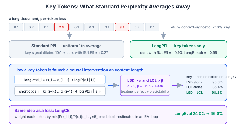
1. The Averaging-Out Failure
For a sequence $\mathbf{x} = (x_1, \dots, x_n)$ and a model $\theta$, standard perplexity is
\[\mathrm{PPL}_{\theta}(\mathbf{x}) = \exp\left(-\frac{1}{n}\sum_{i=1}^{n} \log P_{\theta}(x_i \mid x_{<i})\right) = P_{\theta}(\mathbf{x})^{-1/n}.\]The $1/n$ is the problem. Natural language distributes predictive information extremely unevenly:
- Context-agnostic tokens — grammar, local syntax, boilerplate, common collocations. Typically >90% of a document. A 64-token window predicts these nearly as well as a 32K one.
- Context-dependent (“key”) tokens — entity names, numerals, rare terms, facts that were introduced thousands of tokens earlier. Typically <10%.
Uniform averaging means the 90% drowns the 10%. A model whose long-range retrieval has completely collapsed still scores excellent perplexity, because it still nails the local structure:
Standard PPL — averages over ALL tokens equally
  [non-key 0.1] → [non-key 0.2] → [KEY 2.5] → [non-key 0.1]     mean ≈ 0.72
  The one token that measures long-context ability is diluted 10:1.

LongPPL — evaluate only on key tokens
                   ======> [KEY 2.5] <======
  Directly measures whether the long context was used at all.
Stated as an estimator problem: standard PPL is a low-variance estimate of the wrong quantity. You want expected loss conditioned on long-range dependence; you are computing the marginal, and the conditioning event has ~10% mass.
2. Finding Key Tokens by Causal Intervention
To compute perplexity over key tokens you must first identify them — and on an unlabeled natural corpus there are no annotated “answer” tokens. The paper’s solution is a causal intervention on context length.
Long-Short Difference (LSD)
For each token $x_i$, define two contexts:
- Treatment (long): $l_i = (x_1, \dots, x_{i-1})$ — the full history.
- Control (short): $s_i = (x_{i-K}, \dots, x_{i-1})$ — truncated to a window $K$ (default $K = 4096$).
The Long-Short Difference is
\[\mathrm{LSD}_{\theta}(x_i) = \log P_{\theta}(x_i \mid l_i) - \log P_{\theta}(x_i \mid s_i).\]Under the Rubin causal model, $s_i$ is the counterfactual in which long-range history was ablated, so LSD is the individual treatment effect of the long context on predicting $x_i$. High LSD ($> 2$) means the token genuinely consumes distant information; $\mathrm{LSD} \approx 0$ means local context suffices.
This is the right instrument because it’s interventional, not correlational. Attention weights, gradient saliency, and loss magnitude all tell you where the model is looking or struggling. Cutting the context and re-measuring tells you what it is actually using.
The confounder, and why LCL is needed
LSD alone has a failure mode: some tokens are intrinsically unpredictable — a topic switch, a creative flourish, a typo. For these, $P_\theta(x_i \mid l_i)$ is tiny but $P_\theta(x_i \mid s_i)$ is tinier still, producing a large LSD that reflects noise, not retrieval.
The filter is the Long-Context Likelihood:
\[\mathrm{LCL}_{\theta}(x_i) = \log P_{\theta}(x_i \mid l_i).\]Thresholding on LCL keeps only tokens that are actually predictable once you have the context. LSD asks “does the long context help?”; LCL asks “does it help enough to reach a token the model can get right?” You need both.
Validation on labeled data
On LongEval, where answer tokens are known, key/non-key classification accuracy:
| Selector | Accuracy |
|---|---|
| Random guess | 27.0% |
| LCL alone | 35.4% |
| LSD alone | 85.6% |
| LSD + LCL | 98.2% |
LCL alone is barely above chance — as expected, since “hard to predict” and “needs long context” are different properties. But as a filter on top of LSD it converts a good detector into a near-perfect one.
3. The LongPPL Metric
Given a model $\theta$ under evaluation and a frozen evaluator $\theta_0$ that defines the key tokens:
\[\mathrm{LongPPL}(\mathbf{x}; \theta, \theta_0) = \exp\left(\sum_{i=1}^{n} -\hat{I}(x_i; \theta_0)\, \log P_{\theta}(x_i \mid x_{<i})\right),\]with the hard key-token indicator
\[I(x_i; \theta_0) = \begin{cases} 1, & \mathrm{LSD}_{\theta_0}(x_i) > \alpha \ \text{ and } \ \mathrm{LCL}_{\theta_0}(x_i) > \beta,\\ 0, & \text{otherwise}, \end{cases} \qquad \hat{I}(x_i; \theta_0) = \frac{I(x_i; \theta_0)}{\sum_{j=1}^{n} I(x_j; \theta_0)}.\]Defaults: $\alpha = 2$, $\beta = -2$, $K = 4096$. The metric is notably insensitive to these — Pearson correlation with downstream benchmarks stays below $-0.8$ across the sweep:
| Setting | LongBench | LongEval | RULER |
|---|---|---|---|
| $\alpha = 2, \beta = -2$ | $-0.96$ | $-0.90$ | $-0.90$ |
| $\alpha = 2, \beta = -1$ | $-0.92$ | $-0.94$ | $-0.96$ |
Why the evaluator must be external
The obvious simplification — use the evaluated model as its own key-token selector, $\theta_0 = \theta$ — breaks the metric, and the reason is structural rather than incidental.
A model with a weak long-context window produces $P_\theta(x_i \mid l_i) \approx P_\theta(x_i \mid s_i)$ almost everywhere, because it isn’t using the distant history in the first place. So its LSD is near zero everywhere, it registers essentially no key tokens, and it grades itself on a degenerate token set. Self-evaluation is circular: the very deficiency you want to measure is what disables the measuring instrument. Table 6 in the paper shows the resulting scores go flat across models of wildly different quality.
So you need a strong external evaluator (Qwen2-72B-Instruct, or even Llama-3.1-8B) to fix a consistent set of key tokens across all models being compared. Note the useful consequence: the key-token set is a property of the data plus evaluator, not of the model under test, so it can be computed once and reused — which makes LongPPL a genuinely comparable leaderboard metric rather than a per-model score.
4. Making It Affordable
Computing LSD needs $P_\theta(x_i \mid s_i)$ for $n - K$ tokens. Naively that’s $n-K$ separate forward passes over contexts of length $K$: $\mathcal{O}\big((n-K)K^2\big)$. With $K = 4096$, $K^2 \approx 16.7\text{M}$ against $n \approx 32\text{K}$ — hopeless.
Sliding-window contrastive inference
Introduce a stride $d \le K$ (default $d = 1024$) and batch tokens into chunks of size $d$. For every token $x_{kd + i’}$ in chunk $k$ (with $0 \le i’ < d$), align all their short contexts to the same start index $kd - K$:
\[s_{kd + i'} = (x_{kd - K}, \dots, x_{kd + i' - 1}).\]Because every token in the chunk shares a starting point, ordinary causal masking gives all $d$ conditional probabilities from a single forward pass of length $K + d$:
Naive:
  x_i     ← context [x_{i-K} … x_{i-1}]   → forward pass of length K
  x_{i+1} ← context [x_{i-K+1} … x_i]     → forward pass of length K
  … repeated (n-K) times.

Sliding window (stride d):
  one forward pass of length K + d starting at index kd-K
  → yields conditionals for x_{kd}, …, x_{kd+d-1} in parallel.
Cost drops to
\[\mathcal{O}\!\left(\frac{(n-K)(K+d)^2}{d}\right),\]which in practice makes LongPPL with a Llama-3.1-8B evaluator only 3–4× the cost of a plain single-pass PPL. The trade is a slightly longer effective short context for tokens late in a chunk (up to $K + d$ instead of $K$) — a bounded, uniform bias, and the ablations show the metric doesn’t care.
Tokenizer alignment between evaluator and evaluatee
When $\theta_0$ and $\theta$ use different tokenizers, key-token indices don’t transfer. The paper resolves it in character space: decode the evaluator’s key tokens $X \subseteq x$ to a character set $T = \mathrm{decode}{\theta_0}(X)$, then take the evaluated model’s key set $X’$ to be the maximal subset of $x’ = \mathrm{encode}\theta(t)$ with
\[\mathrm{decode}_{\theta}(X') \subseteq T.\]Only tokens covering the same character spans are compared. This is the same byte-boundary reconciliation problem that shows up in cross-tokenizer on-policy distillation — the maximal-subset rule here is the conservative sibling of the minimal-aligned-unit construction there.
5. From Metric to Objective: LongCE
If key tokens determine long-context ability, standard cross-entropy has the same dilution bug as standard perplexity — gradients are dominated by tokens that teach nothing about long-range retrieval.
LongCE reweights:
\[\mathrm{LongCE}(\mathbf{x}; \theta) = -\frac{1}{n}\sum_{i=1}^{n} I_{\text{soft}}(x_i; \theta)\, \log P_{\theta}(x_i \mid x_{<i}),\]with a differentiable weight built from the same likelihood ratio, clipped:
\[I_{\text{soft}}(x_i; \theta) = \min\big(\exp(\mathrm{LSD}_{\theta}(x_i)),\, \gamma\big) = \min\left(\frac{P_{\theta}(x_i \mid l_i)}{P_{\theta}(x_i \mid s_i)},\, \gamma\right), \qquad \gamma = 5 \text{ (default)}.\]Behavior: if long and short context agree, $I_{\text{soft}} \approx 1$ and the token is trained normally. If the long context massively helps, the weight scales up to $\gamma$. The clip is doing real work — an unclipped likelihood ratio is unbounded above and will blow up the gradient on a handful of outlier tokens. (The same clipped-ratio device appears in PPO-style objectives for the same reason; see First-Order Approximation for Stable LLM-RL Training.)
EM bootstrapping
Training does not use an external evaluator — the joint forward passes would be prohibitive. The model weights itself, giving an EM-style loop:
- E-step: the current $\theta$ computes the long–short difference and estimates $I_{\text{soft}}$ — which tokens are key.
- M-step: $\theta$ minimizes the weighted LongCE, concentrating gradient on those tokens.
As long-context ability improves, key-token estimation sharpens, which sharpens the weighting. Note the asymmetry with §3: self-evaluation was fatal for measurement but is fine for training. Measurement needs a fixed, model-independent token set to be comparable across models; training only needs the weighting to be better than uniform and to improve monotonically. A weak model’s flat $I_{\text{soft}} \approx 1$ degenerates to plain CE — a safe floor, not a collapse.
6. Results
Correlation with downstream benchmarks
Pearson correlation between perplexity variants on GovReport and benchmark scores (more negative = better; lower PPL should mean higher accuracy):
| Metric | LongBench | LongEval | RULER |
|---|---|---|---|
| Standard PPL | $-0.18$ | $+0.24$ | $+0.27$ |
| LongPPL (soft) | $-0.43$ | $-0.23$ | $-0.19$ |
| LongPPL (hard, default) | $\mathbf{-0.96}$ | $\mathbf{-0.90}$ | $\mathbf{-0.90}$ |
Standard PPL is positively correlated on two of three benchmarks — worse than uninformative. The soft variant helps but doesn’t reach the hard indicator; keeping a down-weighted tail of non-key tokens reintroduces the dilution the metric was designed to remove.
LongCE fine-tuning (Llama-2-7B on PG-19 and Pile-arxiv, 200 steps)
| Benchmark | CE | LongCE | Δ |
|---|---|---|---|
| LongEval (acc %) | 24.0 | 46.0 | +22.0 |
| RULER (score %) | 42.7 | 49.7 | +7.0 |
| LongBench (avg %) | 26.9 | 28.2 | +1.3 |
The spread across benchmarks is informative: LongEval is nearly pure retrieval and gains hugely, LongBench mixes in tasks that lean on general ability and gains modestly. LongCE is a targeted intervention on retrieval, and the results say exactly that.
Needle-in-a-Haystack
Beyond 32K, CE-trained models degrade fast — perfect 10/10 on only 2 of 6 configurations at 40K. LongCE models hold near-perfect retrieval, 10/10 on 5 of 6 at 40K, and extend better when RoPE base extension (to 2M) is applied afterwards. Worth noting the composition: the weighting improves how well the model uses its window, which is orthogonal to positional-encoding tricks that extend the window. See GLM-5.2’s 1M-context work for the architectural side of the same problem.
No short-context regression
Average over MMLU, ARC-Challenge, RACE, BBH, TruthfulQA, CommonsenseQA:
| Model | Avg |
|---|---|
| Llama-2-7B baseline | 38.6% |
| CE fine-tuned | 36.9% |
| LongCE fine-tuned | 36.9% |
LongCE costs nothing relative to plain CE here. Both fine-tunes lose ~1.7 points against the base model, so long-context fine-tuning does have a general-ability tax — LongCE just doesn’t add to it.
7. Takeaways
1. Standard PPL on long documents measures local grammar, not long-range retrieval. The $1/n$ average is the bug. With a $+0.27$ correlation on RULER, it is not a weak proxy — it is anti-correlated noise. Stop reporting it as a long-context signal.
2. Cut the context and re-measure. The long–short difference is a clean interventional probe, and LSD + LCL reaches 98.2% key-token identification with no labels. That combination — causal ablation plus a predictability filter — generalizes well beyond context length to any “is the model using capability X?” question.
3. The self-evaluation asymmetry is the subtle part. A model can’t be trusted to identify its own key tokens for measurement (the deficiency disables the instrument) but can for training (the worst case degenerates to uniform CE). Same estimator, opposite verdicts, because comparability and improvement are different requirements.
4. Weighted training is hard-token mining for context length. Up to 90% of long-context fine-tuning compute goes to tokens that teach nothing about long-range dependence. LongCE redirects it for a clipped-ratio weight and one extra truncated forward pass — +22 points on LongEval at 200 steps, with no short-context tax beyond what plain CE already costs.
The wider point connects to how we think about training objectives generally (Why Cross-Entropy Wins): cross-entropy is the right scoring rule, but the uniform token weighting bolted onto it is a convention, not a theorem. Where the capability you care about lives in a sparse subset of positions, the uniform average is actively working against you — in the loss and in the metric alike.