Breaking the Tokenizer Barrier: Cross-Tokenizer On-Policy Distillation
Reading notes on:
- SimCT: Recovering Lost Supervision for Cross-Tokenizer On-Policy Distillation
- Breaking the Tokenizer Barrier: On-Policy Distillation across Model Families
- Cross-Tokenizer On-Policy Distillation via Byte-Prefix Marginalization
On-policy distillation fixes the exposure-bias problem of offline SFT-on-teacher-traces by training the student on its own rollouts and scoring them token-by-token against the teacher. That works beautifully — as long as you quietly accept one assumption that nobody writes down: teacher and student share a tokenizer.
The moment you distill Qwen → Llama, or GLM → Gemma, the assumption dies twice over:
- Vocabulary mismatch ($V_T \neq V_S$). The two next-token distributions live over different simplices. There is no coordinate-wise KL to compute.
- Segmentation mismatch ($\text{len}_T \neq \text{len}_S$). Even on identical text, the two tokenizers cut the byte stream at different boundaries, so position $t$ on one side does not correspond to position $t$ on the other.
The naive workaround — SimpleOPD, keep only the positions where both tokenizers happen to emit the exact same surface token — throws away 40–50% of the teacher’s supervision. Three papers from mid-2026 attack this from three genuinely different angles. This note walks the math of each and then compares them on the axes that actually matter.
This is a direct sequel to Revisiting On-Policy Distillation and SOPD; the multi-teacher variant of the same problem is in Open-MOPD.
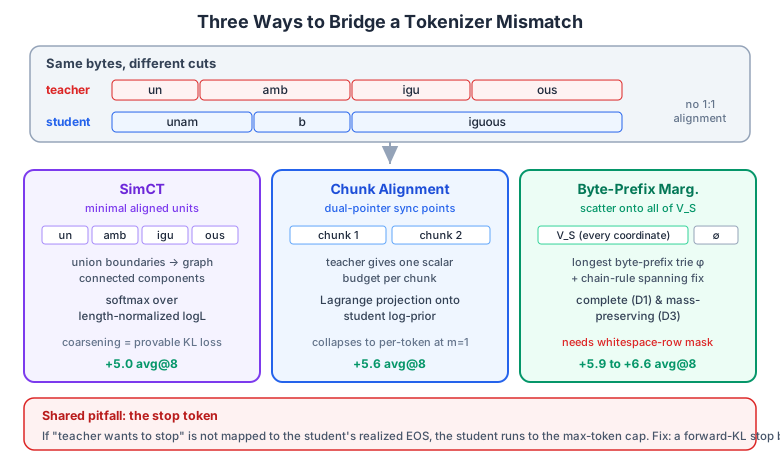
1. One Frame: The Common Supervision Space
All three methods are instances of the same generalization. Instead of matching token-to-token, construct a common supervision space $\mathcal{U}$ and push both models into it via scoring maps $\Pi_T, \Pi_S$. At a student-generated prefix $x_{<t}$:
\[q_T(\cdot \mid x_{<t}) = \Pi_T\big(p_T(\cdot \mid x_{<t})\big) \in \Delta(\mathcal{U}), \qquad q_S(\cdot \mid x_{<t}) = \Pi_S\big(p_S(\cdot \mid x_{<t})\big) \in \Delta(\mathcal{U}).\]Distillation then runs entirely inside $\mathcal{U}$:
\[\mathcal{L}_{\text{gOPD}}(x_{<t}) = \mathcal{D}\big(q_S(\cdot \mid x_{<t}),\, q_T(\cdot \mid x_{<t})\big),\]with $\mathcal{D}$ typically reverse-KL. Everything reduces to one design question: how do you build $\mathcal{U}$ so that it retains the most teacher signal while staying mathematically well-formed?
- SimCT makes $\mathcal{U}$ the set of minimal jointly-tokenizable text spans.
- Chunk alignment makes $\mathcal{U}$ local: it projects a chunk-level teacher budget back onto student tokens.
- BPM makes $\mathcal{U}$ the entire student vocabulary $V_S$, plus a residual bucket.
2. SimCT: Minimal Aligned Units
Sun et al. (May 2026) expand the supervision space past exact token overlap with minimal aligned units — the finest text spans on which both tokenizers agree about the boundaries.
Graph construction
Take a text span $y$. The teacher tokenizer induces a partition $P_T(y) = {[b_{i-1}^T, b_i^T)}{i=1}^m$ over byte indices; the student induces $P_S(y) = {[b{j-1}^S, b_j^S)}_{j=1}^n$. Then:
- Union the boundary sets: $B_\cup(y) = B_T(y) \cup B_S(y)$.
-
Sort into $0 = c_0 < c_1 < \dots < c_\ell = y $, giving atomic fragments $A(y) = {[c_{k-1}, c_k)}_{k=1}^{\ell}$. - Build an undirected graph $G_y$ on those fragments. Connect two fragments if they fall inside the same teacher token or the same student token.
- The connected components of $G_y$ are the minimal aligned units:
Each $u_k$ is the shortest character run that is boundary-consistent under both tokenizers. Nothing finer is jointly tokenizable — that is the content of SimCT’s Theorem 1.
Scoring maps
The supervision space is $\mathcal{U}{\text{SimCT}} = (V_T \cap V_S) \cup \mathcal{A}$. For each $u \in \mathcal{U}{\text{SimCT}}$ and each model $M \in {T, S}$:
- For a shared 1:1 token $u \in V_T \cap V_S$, use the plain next-token log-probability:
- For a multi-token unit $u \in \mathcal{A}$ realized as $\tau_M(u) = (v_1, \dots, v_k)$ under tokenizer $M$, use the length-normalized average log-likelihood:
Length normalization is what makes a 1-token unit and a 4-token unit comparable on the same scale. Then softmax over the candidate set:
\[q_M^{\text{SimCT}}(u \mid x_{<t}) = \frac{\exp\big(s_M(u \mid x_{<t})\big)}{\sum_{u' \in \mathcal{U}_{\text{SimCT}}} \exp\big(s_M(u' \mid x_{<t})\big)}.\]Why granularity is not a free parameter
SimCT’s Proposition 1 says something sharp: coarsening the units can only destroy signal, never create it.
Proposition 1. Let $q_S^{\min}, q_T^{\min}$ be distributions over minimal aligned units, and let $q_S^{C}, q_T^{C}$ be obtained by any non-trivial coarsening $\mathcal{C}$ that sums probabilities inside each coarse unit. Then
\[\mathrm{KL}\big(q_S^{\min} \,\|\, q_T^{\min}\big) \;\ge\; \mathrm{KL}\big(q_S^{C} \,\|\, q_T^{C}\big).\]Proof. For coarse span $c$, write $Q_M(c) = \sum_{u \in c} q_M^{\min}(u)$ and $q_M^{\min}(u \mid c) = q_M^{\min}(u)/Q_M(c)$. Then
\[\mathrm{KL}(q_S^{\min} \| q_T^{\min}) = \sum_{c} \sum_{u \in c} Q_S(c)\, q_S^{\min}(u \mid c) \log\!\left(\frac{Q_S(c)\, q_S^{\min}(u \mid c)}{Q_T(c)\, q_T^{\min}(u \mid c)}\right).\]Splitting the log into the coarse ratio and the conditional ratio, and using $\sum_{u \in c} q_S^{\min}(u \mid c) = 1$:
\[= \underbrace{\sum_{c} Q_S(c) \log \frac{Q_S(c)}{Q_T(c)}}_{\mathrm{KL}(Q_S \| Q_T)} \;+\; \sum_{c} Q_S(c)\, \mathrm{KL}\big(q_S^{\min}(\cdot \mid c) \,\|\, q_T^{\min}(\cdot \mid c)\big).\]The second term is a convex combination of KLs, hence $\ge 0$. $\blacksquare$
The gap
\[\Delta_{\mathcal{C}} = \sum_{c} Q_S(c)\, \mathrm{KL}\big(q_S^{\min}(\cdot \mid c) \,\|\, q_T^{\min}(\cdot \mid c)\big) \;\ge\; 0\]is the within-unit teacher–student disagreement you erase by going coarse. This is the chain rule for KL, applied as an argument about supervision design: every level of aggregation is a strict information loss unless the two models already agree inside every coarse span. It is the same monotonicity intuition that makes token-level rather than sequence-level objectives the default in the distributional view of post-training.
3. Dual-Pointer Chunk Alignment + Semantic-Prior Credit
Niu et al. (June 2026) take the opposite tack: don’t rebuild the vocabulary, rebuild the alignment, then solve a small constrained optimization to push teacher credit back onto student tokens.
DPCA: finding synchronization points
Two pointers walk the student response $y_S = {s_1, \dots, s_m}$ and the teacher-retokenized counterpart $y_T = {t_1, \dots, t_k}$. Using the detokenizer $D$, compare decoded string lengths:
-
If $ D(y_{S,1:i}) < D(y_{T,1:j}) $ → advance the student pointer $i$. -
If $ D(y_{S,1:i}) > D(y_{T,1:j}) $ → advance the teacher pointer $j$. - If equal → declare a synchronized chunk boundary, emit the chunk, reset, continue.
This is just merge-walking two partitions of the same byte stream, and Theorem 4.2 of the paper gives the property you want: DPCA finds the complete set of synchronization points and the chunks it emits are minimal — none can be subdivided further. Same conclusion as SimCT’s connected components, reached procedurally instead of graph-theoretically.
Chunk-level credit assignment via Lagrange multipliers
Inside a chunk $(s_c, t_c)$, the teacher’s total log-likelihood is a single scalar budget:
\[L_T^{(c)} = \sum_{j=1}^{|t_c|} \log \pi_T(t_{c,j} \mid \cdot).\]We need to spread that budget over the $m$ student tokens in the chunk without destroying the student’s internal semantic structure — its prior $p = {\pi_{\theta_{\text{old}}}(s_i \mid \cdot)}_{i=1}^m$. Formulate it as a least-squares projection in log-space under a sum constraint:
\[\min_q \; \frac{1}{2}\sum_{i=1}^m \big(\log q_i - \log p_i\big)^2 \quad \text{s.t.} \quad \sum_{i=1}^m \log q_i = L_T^{(c)}.\]Lagrangian:
\[\mathcal{L}(q, \lambda) = \frac{1}{2}\sum_{i=1}^m \big(\log q_i - \log p_i\big)^2 + \lambda\left(\sum_{i=1}^m \log q_i - L_T^{(c)}\right).\]Stationarity in $\log q_i$:
\[\frac{\partial \mathcal{L}}{\partial \log q_i} = (\log q_i - \log p_i) + \lambda = 0 \;\;\Longrightarrow\;\; \log q_i = \log p_i - \lambda.\]Summing and applying the constraint, with $L_S^{(c)} = \sum_i \log p_i$:
\[L_S^{(c)} - m\lambda = L_T^{(c)} \;\;\Longrightarrow\;\; \lambda = \frac{L_S^{(c)} - L_T^{(c)}}{m}, \qquad \log q_i = \log p_i - \frac{L_S^{(c)} - L_T^{(c)}}{m}.\]So the exact solution is a uniform additive shift in log-space. The paper then adopts the multiplicative variant instead, which preserves proportional ranking of the student’s prior rather than shifting it flat:
\[\log q_i = \frac{L_T^{(c)}}{L_S^{(c)}} \log p_i.\]The per-token advantage falls out immediately:
\[\hat{A}_{i,t} = \log q_i - \log p_i = \left(\frac{L_T^{(c)}}{L_S^{(c)}} - 1\right)\log p_i.\]Note the sanity check: at $m = 1$ (a genuine 1:1 alignment), $L_S^{(c)} = \log p_1$ and $L_T^{(c)} = \log q_1$, so $\hat{A} = \log q_1 - \log p_1$ — exactly standard per-token distillation. The method degrades gracefully to the same-tokenizer case.
The trade-off relative to SimCT is visible in the formula: the teacher only contributes a scalar per chunk. Within-chunk shape comes entirely from the student’s own prior. That is cheap and stable, but it is strictly less teacher information than SimCT’s full unit-level distribution.
Sample efficiency
The paper’s Figure 2 is the number worth remembering. To hit 44.4% on AIME24:
| Route | Extra data | Compute |
|---|---|---|
| Offline SFT | ~482K teacher-supervised examples | $1.17 \times 10^{21}$ FLOPs |
| Cross-tokenizer OPD | ~20K training prompts | $4.8 \times 10^{19}$ FLOPs |
That is a 24.1× compute reduction for the same accuracy — consistent with the general finding that dense per-token feedback dominates sparse trajectory-level supervision, which is the same lesson as privileged value functions in RL.
4. Byte-Prefix Marginalization
Wang et al. (July 2026) go furthest: build a target over the full student vocabulary. BPM states three design requirements up front:
- (D1) Vocabulary completeness — the target is defined on every coordinate of $V_S$.
- (D2) Byte-level alignment — mapping is decided purely by byte representation.
- (D3) Mass preservation — no teacher probability is discarded; the target sums to exactly $1$.
The longest-prefix map
Different tokenizers must decode to the same bytes. Precompute a static map $\phi: V_T \to V_S \cup {\bot}$ sending each teacher token to the longest student token that is a byte-prefix of it:
\[\phi(w) = \operatorname*{argmax}_{u \in V_S,\; \text{bytes}(u) \preceq \text{bytes}(w)} |\text{bytes}(u)|,\]with $\bot$ when no student token prefixes $w$. This is one trie lookup per teacher token, built once, reused for the whole run. Then scatter the teacher’s next-token distribution $q_{j(i)}$ onto $V_S$:
\[t_i(u) = \sum_{w:\, \phi(w) = u} q_{j(i)}(w), \qquad t_i(\emptyset) = \sum_{w:\, \phi(w) = \bot} q_{j(i)}(w).\]The explicit residual bucket $\emptyset$ is what buys (D3): mass that has nowhere to go is named, not dropped. That distinction matters — a target that silently loses 5% of its mass is a differently-normalized target, and the student will chase the renormalization artifact.
Spanning tokens and the chain-rule correction
A student token can swallow several teacher tokens. Classic case: the student has </think> as one token while the teacher emits </, think, >. Scattering only at the aligned position gives that student token near-zero mass, so the student is actively taught not to close its thinking block. BPM fixes it with a chain-factorized correction:
where $w_k^t$ is the realized teacher token at step $k$ and
\[\pi_{j+m}(r) = \sum_{w \in V_T:\; r \preceq \text{bytes}(w)} q_{j+m}(w)\]is the total teacher prefix mass on the remaining bytes $r$ of the final partial token. In words: the probability the teacher “would have produced” the student’s long token is the product of the teacher steps that realize it, times the prefix mass of whatever tail is left over.
The failure mode nobody predicted: indentation collapse
High-fidelity byte alignment turns out to be too faithful on code. Whitespace is syntax in Python, and at all-whitespace positions a byte-exact target transfers tokenizer segmentation preferences rather than semantics. If the teacher likes emitting an 8-space indent as two \t tokens and the student prefers eight literal spaces, BPM dutifully penalizes the student for a choice that carries no meaning.
The result is dramatic: GLM-Z1-9B distillation saw code pass@8 fall from 49% to 9%.
The fix is a one-line whitespace-row mask — if the student’s realized token at row $i$ is entirely spaces/tabs, withhold the target at that position. It touches only ~3.5% of aligned code rows, and it takes block-level indentation errors from 84% to 0%.
This is worth generalizing beyond BPM: the more literally your supervision signal is grounded in bytes, the more aggressively it transfers representational choices along with behavioral ones. Anywhere the two tokenizers make an arbitrary encoding choice over semantically identical bytes, the distillation target is pure noise. Related pathologies from the tokenizer side are in Tokenizer Learning; the same “mask the positions that carry no signal” move, applied to evaluation and loss weighting instead of distillation, is LongPPL / LongCE.
5. Comparison
| Dimension | SimCT (May 2026) | Chunk Alignment (Jun 2026) | BPM (Jul 2026) |
|---|---|---|---|
| Supervision unit | Minimal aligned units (finest jointly-tokenizable spans) | Greedy synchronized chunks (dual-pointer) | Full student vocabulary via byte-prefix map |
| Space $\mathcal{U}$ | $(V_T \cap V_S) \cup \mathcal{A}$ | Local chunk projection onto student tokens | $V_S$ + explicit residual $\emptyset$ |
| Transformation | Softmax over length-normalized log-likelihood | Proportional log-space scaling (Lagrange) | Longest-prefix scatter + chain-rule spanning fix |
| D1 vocab completeness | No — unmatched vocabulary gets no signal | No — scores live on chunk subsets | Yes |
| D2 byte alignment | Yes | Yes | Yes (deterministic trie) |
| D3 mass preservation | No | No | Yes |
| Whitespace stability | Stable (ignores unaligned sub-token noise) | Stable (chunk constraint averages it out) | Unstable without whitespace-row mask |
| Avg@8 gain (reasoning) | +5.0 | +5.6 | +5.9 to +6.6 |
Three things I’d take away
1. Granularity is the whole ballgame, and it has a proof. SimCT’s Proposition 1 and DPCA’s minimality theorem are the same claim from two directions: transfer at the finest synchronization boundary you can construct. Every coarsening step is a provable KL loss equal to the within-span disagreement — exactly the disagreement you were trying to distill.
2. There is a real completeness/robustness trade. BPM wins on benchmarks precisely because it satisfies D1 and D3 — every student coordinate gets a target and no mass is thrown away. But that same literalism is what produced indentation collapse. SimCT and chunk alignment are less complete and, for that reason, accidentally more robust: they never had a target for the noisy positions in the first place. BPM has to earn robustness back with a mask.
3. Don’t forget the stop token. All three papers hit the same operational wart: if “the teacher wants to stop here” isn’t explicitly mapped to the student’s realized EOS, the student runs to the max-token cap and inference latency explodes. The fix is a stop bridge — an explicit forward-KL ($D_0$) endpoint on the stop decision, so a healthy stop gradient survives even when the student’s EOS probability has initially collapsed. Reverse-KL is mode-seeking and will happily let a near-zero EOS probability stay near-zero; forward-KL will not.
The through-line with SOPD and Open-MOPD is that on-policy distillation is quietly becoming a supervision-interface design problem rather than a loss-function problem. You already know you want dense, on-policy, token-level feedback. The open question is what object you compute that feedback over — steps, teachers, or, here, byte spans. And once the tokenizer barrier falls, distillation stops being an intra-family compression trick and becomes a way to move capability across the entire open-weights ecosystem.