Mixture-of-Recursions: Learning Dynamic Recursive Depths per Token
Reading notes on:
Efficiency work on Transformers has long split into two lanes that rarely meet. Parameter efficiency shrinks the weights, usually by tying layers so the same block is applied repeatedly. Adaptive computation varies the work per input, usually by token routing or early exit. Both are well studied; neither has been the other’s natural home.
Mixture-of-Recursions (MoR) puts them in the same architecture: token-level conditional compute inside a weight-tied recursive Transformer. The result is a three-way saving: fewer unique parameters (up to $\sim 3\times$), fewer FLOPs per easy token, and a KV cache that shrinks with the routing distribution rather than staying dense.
This is the token-adaptive branch of the depth-recurrence family. The compute-matched scaling-law branch is the subject of tomorrow’s post on SMELT, and the theory-of-computation angle is in Looped Transformers.
1. Parameter Sharing: Which Tying Scheme?
A standard non-recursive Transformer with $L$ unique layers evolves token $t$ as
\[\mathcal{H}^{\ell+1}_t = f\!\left(\mathcal{H}^\ell_t; \Phi_\ell\right), \qquad \ell \in \{0, \dots, L-1\}\]with $f$ the block and $\Phi_\ell$ its distinct parameters. Recursive models partition the network into $N_r$ recursion blocks sharing a parameter pool $\Phi’$: unrolled depth stays $L$, unique parameter blocks drop by $N_r$.
Four candidate unrolling schemes:
1. Cycle:           [(0, 1, 2), (0, 1, 2), (0, 1, 2)]
2. Sequence:        [(0, 0, 0), (1, 1, 1), (2, 2, 2)]
3. Middle-Cycle:    [0, (1, 2), (1, 2), (1, 2), 3]     <-- MoR default
4. Middle-Sequence: [0, (1, 1, 1), (2, 2, 2), 3]
Cycle indexes the parameter block cyclically:
\[\mathcal{H}^{\ell+1}_t = f\!\left(\mathcal{H}^\ell_t; \Phi'_{\ell \bmod (L/N_r)}\right)\]Pushing hidden states through the same cyclic sequence encourages loop-like iterative refinement: “rethink the problem” rather than “apply another transformation.”
Sequence applies each unique block consecutively:
\[\mathcal{H}^{\ell+1}_t = f\!\left(\mathcal{H}^\ell_t; \Phi'_{\lfloor \ell/N_r \rfloor}\right)\]Back-to-back identical layers hit diminishing returns and redundant feature learning quickly.
Middle-Cycle, the default, keeps the first and last layers unshared and cycles the interior:
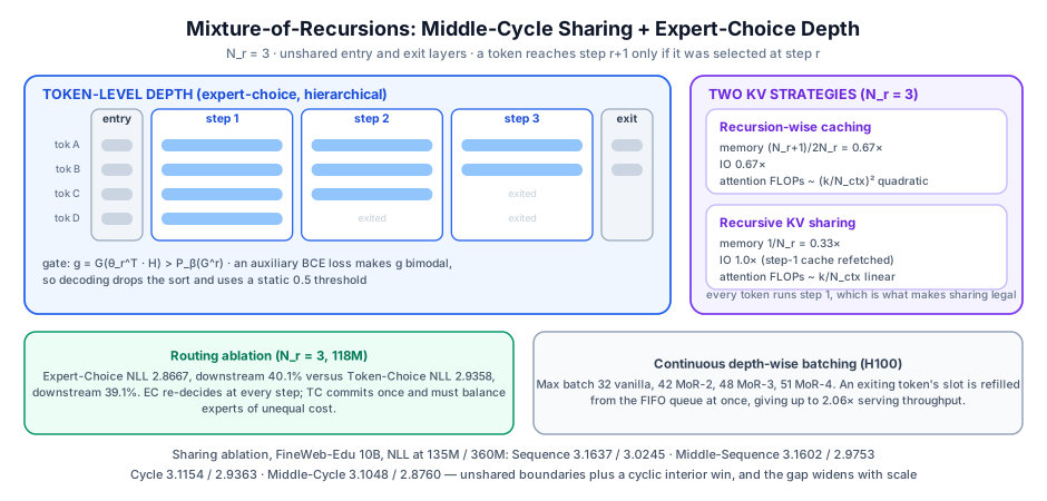
\[\mathcal{H}^1_t = f\!\left(\mathcal{H}^0_t; \Phi_0\right)\] \[\mathcal{H}^{\ell+1}_t = f\!\left(\mathcal{H}^\ell_t; \Phi'_{\left((\ell - 1) \bmod \frac{L-2}{N_r}\right) + 1}\right), \quad \ell \in \{1, \dots, L-2\}\] \[\mathcal{H}^L_t = f\!\left(\mathcal{H}^{L-1}_t; \Phi_{L-1}\right)\]Dedicated entry and exit layers give the network capacity for embedding adaptation and vocabulary prediction respectively, the two jobs that are least like “iterative refinement” and therefore worst served by shared weights. Middle-Sequence is the same boundary treatment with sequence-based interior sharing.
Ablation on FineWeb-Edu (10B tokens):
| Strategy | 135M base ($N_r=3$) NLL | 360M base ($N_r=3$) NLL |
|---|---|---|
| Sequence | 3.1637 | 3.0245 |
| Middle-Sequence | 3.1602 | 2.9753 |
| Cycle | 3.1154 | 2.9363 |
| Middle-Cycle | 3.1048 | 2.8760 |
Both effects are real and additive: cycling beats sequencing, and unshared boundaries beat fully shared. The gap widens at 360M, which is the encouraging direction. Note that SMELT converges on the same Prelude–Recur–Coda layout independently.
2. Routing: Expert-Choice vs. Token-Choice
MoR must decide how many times each token passes through the shared block. Two gating mechanisms, with genuinely different failure modes.
2.1 Expert-Choice routing
Each recursion depth acts as an expert selecting the top-$k$ most important tokens from the batch. At step $r$, the hidden state is projected through routing parameters $\theta_r$:
\[g^r_t = \mathcal{G}\!\left(\theta_r^\top \mathcal{H}^r_t\right)\]with $\mathcal{G}$ typically a sigmoid. Hierarchical filtering enforces that a token can be selected at step $r+1$ only if it was selected at step $r$, which mimics physical early exit and prevents information bypass.
\[\mathcal{H}^{r+1}_t = \begin{cases} g^r_t\, f(\mathcal{H}^r_t, \Phi') + \mathcal{H}^r_t, & \text{if } g^r_t > P_\beta(G^r) \\[4pt] \mathcal{H}^r_t, & \text{otherwise} \end{cases}\]where $P_\beta(G^r)$ is the $\beta$-percentile threshold over routing scores across the batch. Top-$k$ by construction gives a static, predictable compute budget, a real operational advantage over token-choice, where per-batch cost fluctuates.
The causality problem. Top-$k$ requires sorting scores across the whole sequence, but autoregressive decoding doesn’t have the future tokens. Two mitigations:
-
Auxiliary router. A lightweight classifier trained jointly to predict whether a token’s raw score will cross the top-$k$ threshold, supervised by the actual selections of the causal main router:
\[\mathcal{L}_{\text{AuxRout}} = -\sum_t \left[ y_t \log \hat{y}_t + (1-y_t)\log(1-\hat{y}_t)\right]\]Gradients are blocked from flowing back into the main hidden states, so the auxiliary objective cannot degrade the primary representations.
-
Auxiliary loss (selected). Skip the extra network; regularize the primary router directly to be bimodal:
\[\mathcal{L}_{\text{Aux}} = \gamma \cdot \text{BCE}(G^r, Y^r)\]Once raw outputs cluster near 0.0 and 1.0, inference can drop sorting entirely and use a static threshold ($g^r_t > 0.5$). The paper’s Figures 5b and 9a show the auxiliary-loss variant achieving clean separation between selected and unselected tokens, which is what makes the static threshold stable.
The second option wins because it removes a component rather than adding one: the sorting operation, the training/inference mismatch, and the extra classifier all disappear together.
2.2 Token-Choice routing
Each token commits to a fixed recursion depth up front. From the post-first-layer state $\mathcal{H}^1_t$:
\[\mathbf{g}_t = \text{Softmax}\!\left(\Theta^\top \mathcal{H}^1_t\right), \qquad \mathbf{g}_t \in \mathbb{R}^{N_r}\]Assignment is $i = \arg\max_j g_{jt}$, and the update is
\[\mathcal{H}^{r+1}_t = \begin{cases} g^r_t\, f(\mathcal{H}^r_t, \Phi') + \mathcal{H}^1_t, & \text{if } r = i \\[4pt] g^r_t\, f(\mathcal{H}^r_t, \Phi'), & \text{otherwise} \end{cases}\]No causality violation, but load imbalance, and experts that receive no tokens collapse. Two standard MoE remedies apply:
Explicit balancing loss:
\[\mathcal{L}_{\text{Balance}} = \alpha \sum_{i=1}^{N_r} f_i P_i\]with $f_i = \frac{N_r}{T}\sum_{t=1}^{T} \mathbb{I}(\text{token } t \text{ selects expert } i)$ the routed fraction and $P_i = \frac{1}{T}\sum_{t=1}^{T} g_{it}$ the mean routing score.
Loss-free router biasing adds per-expert bias terms adjusted each batch by load violation:
\[e_i = c_i - \bar{c}_i, \qquad b_i \leftarrow b_i + u \cdot \text{sign}(e_i)\]where $c_i$ is the assigned token count, $\bar{c}_i$ the balanced target, and $u$ the update rate.
Which wins
At $N_r=3$, 118M parameters:
- Expert-Choice: validation NLL 2.8667, average downstream accuracy 40.1%
- Token-Choice: validation NLL 2.9358, average downstream accuracy 39.1%
EC’s advantage is granularity: it re-decides at every recursion step instead of committing once. A token whose difficulty only becomes apparent after one pass can still be escalated. Token-choice has to guess from the embedding.
There’s a deeper reason token-choice struggles here that doesn’t apply to ordinary MoE: the experts are structurally heterogeneous. Expert 1 performs one recursion, expert 2 performs two. Balancing loads across experts of unequal cost is a different and harder problem than balancing across symmetric FFN experts, which is why it needs heavy z-loss and warmup. Contrast with the symmetric-expert balancing in UltraEP and RoutePack.
3. KV Cache Dynamics
Dynamic depth breaks KV caching in a way early-exit models never solved cleanly: if a token exits early, its keys and values at deeper layers don’t exist, and subsequent tokens’ causal attention has holes. MoR offers two answers at different points on the memory/IO curve.
3.1 Recursion-wise caching
Only tokens routed to a given recursion step store KV entries at that level, and attention at that level is confined to the active subset.
Token 1 (routes to step 3):  [KV1] [KV2] [KV3]   all cached
Token 2 (routes to step 1):  [KV1]   --    --    only first cached
Attention for later queries is restricted to locally active tokens.
Assuming balanced routing capacity $\frac{N_r}{N_r}, \frac{N_r-1}{N_r}, \dots, \frac{1}{N_r}$, normalized against vanilla:
- KV memory: $\frac{N_r + 1}{2N_r}$ → 0.67× at $N_r=3$
- KV IO: $\frac{N_r + 1}{2N_r}$ → also 0.67×
- Attention FLOPs: quadratic reduction, $\left(\frac{k}{N_{\text{ctx}}}\right)^2$ per layer
3.2 Recursive KV sharing
Because Middle-Cycle guarantees every token processes at least the first recursion block, MoR can cache KV only at step 1 and reuse it globally at all depths.
All prior tokens' keys/values cached at step 1 only.
Step 2 and step 3 queries skip projection and attend to the step-1 cache.
- KV memory: $\frac{1}{N_r}$ → 0.33× at $N_r=3$
- KV IO: 1.0× (the global step-1 cache must be fetched at every depth)
- Attention FLOPs: linear reduction, $\frac{k}{N_{\text{ctx}}}$
The trade is explicit and worth stating plainly: recursive sharing halves memory again but gives back all the IO savings. On a memory-capacity-bound deployment that’s a clear win; on a bandwidth-bound decode it is not. Which regime you’re in is exactly the roofline question from Efficiency in LLMs.
3.3 Why sharing doesn’t collapse
Sharing projection matrices across depths should risk representational collapse. The paper’s probe of a pretrained recursive model says otherwise:
- Hidden states grow steadily in $L_2$ norm across unrolled layers.
- Key and value states show cosine similarity close to 1.0 along the diagonals of different recursion stages.
The projections naturally learn to align and stabilize signal scale across depths, which is why KV sharing costs only a minor perplexity drop. This is the same phenomenon SMELT measures from the other side, finding second-pass Q/K similarity ~0.90 against V similarity ~0.70: high agreement on where to look, more movement in what is read.
4. Serving: Continuous Depth-Wise Batching
The classic serving bubble is fast queries idling while the batch waits on the slowest one. Because MoR runs one shared parameter block, it supports continuous depth-wise batching: batch token recursion steps, not sequences.
- A token exiting early at step $r < N_r$ vacates its slot in the active batch.
- The scheduler immediately pulls a pending query from the FIFO queue, pre-processes embeddings, and fills the slot.
- Execution streams through the shared block without synchronization barriers.
Smaller KV caches also mean larger batches under fixed VRAM (H100):
| Model | Max batch size |
|---|---|
| Vanilla Transformer | 32 |
| MoR-2 | 42 |
| MoR-3 | 48 |
| MoR-4 | 51 |
Combined with early exit, this yields up to 2.06× serving throughput over optimized vanilla baselines. Structurally it’s the same idea as continuous batching in vLLM V1, moved one level down from the sequence to the recursion step, which is only possible because weight tying makes every depth the same kernel launch.
5. Scaling and Test-Time Behavior
IsoFLOP scaling
Parameter-sharing architectures usually scale badly. Under isoFLOP budgets, MoR’s compute-optimal path is notably flatter than vanilla’s:
Validation Loss
  ^
  |   \
  |    \   Vanilla
  |     \ ------*  (flat slope, data-hungry)
  |      \
  |       *  (star = compute-optimal point)
  |        \
  |         \   MoR
  |          \ ======*  (flatter path, favors model size)
  |
  +--------------------------------------------> Model Size / Parameters
Vanilla models under isoFLOP prefer smaller parameter counts on longer token horizons; they’re data-hungry. MoR prefers the opposite: scale parameters (width) rather than tokens. The quality of the shared recursive block is the binding bottleneck, so MoR favors wide-and-short configurations on less data.
That’s a real deployment consideration, not just a curve shape. If tokens are your scarce resource, MoR’s optimal point is friendlier. Broader treatment of these surfaces in Deconstructing Scaling Laws and The Architecture of Scaling Laws.
Test-time scaling
Because depth is a runtime parameter, MoR can spend more inference FLOPs by unrolling further (no retraining):
Inference quality (log-likelihood)
  ^
  |                     [step 4 refinement] -> -2.85
  |          [step 3 refinement] -> -2.90
  |  [step 2 base] -> -3.05
  |
  +--------------------------------------------> Inference recursion steps
Each additional step refines hidden representations further. This is a latent-space test-time scaling knob, orthogonal to the token-space one analyzed in The Mechanics of Reasoning Effort and Inference Scaling; you deepen the computation per token rather than emitting more thinking tokens.
6. Open Problems
- Heterogeneous expert collapse. Token-choice balancing is structurally harder than in standard MoE because experts differ in cost, not just in specialization. Standard routers don’t converge cleanly; z-loss and warmup are load-bearing.
- Post-training on reasoning data. Latent-space reasoning is the natural fit for a depth-adaptive model, and the obvious next question is how the router learns to allocate depth when fine-tuned on reasoning datasets under GRPO-style RL. Nobody has run that experiment.
- Scaling the unshared block. Below ~135M, the recursive bottleneck degrades quality outright. Past ~3B, the likely fix is more unshared capacity (wider first/last blocks, or LoRA adapters at specific recursion depths) to close the gap with vanilla. The recursion is a prior, and priors need to weaken as data grows.
Takeaways
- Weight tying and adaptive compute are complements, not alternatives. Tying makes every depth the same kernel; adaptive depth makes the tying pay for itself instead of just saving parameters.
- Boundaries matter more than the interior. Middle-Cycle’s unshared entry/exit layers are the single biggest ablation win, and SMELT reaches the same layout from an entirely different direction.
- Expert-choice beats token-choice (NLL 2.8667 vs. 2.9358) because it re-decides per step, and the causality problem is best solved by making the router bimodal rather than by adding a second router.
- The KV story has two settings, not one. 0.67× memory at 0.67× IO, or 0.33× memory at 1.0× IO. Pick by which resource you’re actually short of.
- MoR scales along width, not tokens. Its isoFLOP optimum sits at larger parameter counts than vanilla’s, worth knowing before you assume a shared-weight model is just a smaller model.
Tomorrow: SMELT asks whether looping still wins once you match FLOPs, parameters, and KV cache simultaneously, the control MoR’s isoFLOP analysis only partially imposes.