SMELT: Scaling Laws for Compute-Matched MoE Looped Transformers
Reading notes on:
Looped and weight-tied Transformers have a credibility problem, and it is a measurement problem. Papers in this line (Huginn, Ouro, and others) report gains in parameter efficiency, which is true and also the easy part: of course reusing a layer stack saves parameters. What repeating a stack does not save is FLOPs per token or KV cache, both of which go up. Compare a looped model against a dense baseline at matched parameters and you have quietly given the looped model extra compute and extra memory. Call it FLOPs conflation.
SMELT (Sparse MoE transformer, middle layers Loop Twice) is the attempt to settle the question honestly: match three budgets at once, then fit scaling laws and see whether looping is still ahead. It is. But the interesting content is how the matching is done and why the advantage grows with scale.
This is the compute-matched counterpart to yesterday’s post on Mixture-of-Recursions, which takes the same weight-tied substrate in the token-adaptive direction.
1. The Three-Budget Matching Problem
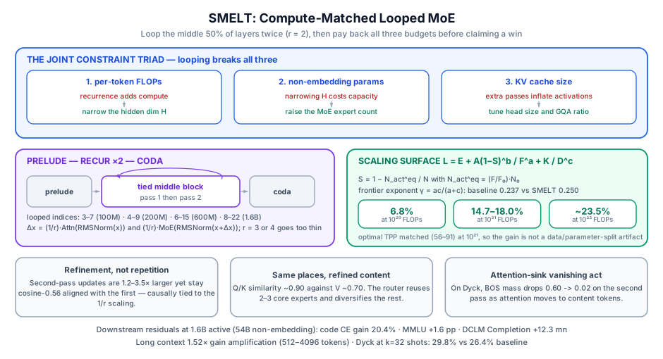
The honest baseline requires parity on what the paper calls the joint constraint triad:
- Per-token training/inference FLOPs
- Total non-embedding parameters
- KV cache size
Looping violates all three in the naive setup. SMELT’s recipe restores parity with three compensating moves:
- Narrow the hidden dimension $H$ to pay back the FLOPs that depth recurrence added.
- Use MoE to recover the lost capacity: sparsity decouples total parameters from per-token compute, so raising the expert count restores parameters without restoring FLOPs.
- Adjust head sizes and GQA ratios to hold KV cache constant.
The MoE step is what makes the whole thing work. Without it, narrowing $H$ enough to pay the FLOPs bill would cost so much capacity that looping could never come out ahead. Sparsity is not an add-on here; it is the mechanism that makes compute-matched looping possible at all.
2. Architecture and the $1/r$ Residual Scaling
SMELT uses a Prelude–Recur–Coda layout: specialized entry layers, a tied middle block, specialized exit layers. (MoR’s Middle-Cycle ablation lands on the same shape from a completely different search, a good sign that the boundary layers are doing real work rather than being a tuning artifact.)
Empirical search says loop the middle 50% of physical layers twice ($r=2$). Concretely, the looped indices are layers 3–7 (100M), 4–9 (200M), 6–15 (600M), and 8–22 (1.6B). Higher recurrence ($r=3$ or $4$) increases effective depth, but the budget-matching constraints then force the model to be so thin that returns go negative: depth bought at the cost of width stops paying.
Residual stream scale compensation
Weight-tied layers receive correlated gradient contributions from multiple points in the execution trace, which destabilizes training. SMELT tempers the per-pass update by $1/r$:
\[\Delta x^{\text{attn}}_l = \frac{1}{r} \cdot \text{Attn}\!\left(\text{RMSNorm}(x_l)\right)\] \[\Delta x^{\text{moe}}_l = \frac{1}{r} \cdot \text{MoE}\!\left(\text{RMSNorm}\!\left(x_l + \Delta x^{\text{attn}}_l\right)\right)\]The stated justification is stabilization, but the mechanistic consequence is more specific and shows up in the probes later: scaling down each pass keeps the second pass directionally aligned with the first, so the loop performs refinement rather than overwriting. The scaling factor is what buys the inductive bias, not just the numerical safety. Related residual-stream engineering appears in Manifold-Constrained Hyper-Connections and Attention Residuals.
3. Compute-Equivalent Sparsity
Parameter-count sparsity is the wrong x-axis when compute and storage are decoupled. SMELT defines a FLOPs-based metric instead:
\[N^{\text{eq}}_{\text{act}} = \frac{F}{F_0} \cdot N_0, \qquad S = 1 - \frac{N^{\text{eq}}_{\text{act}}}{N}\]$F$ is per-token training FLOPs, $N$ is total non-embedding parameters, and $F_0, N_0$ come from the dense control baseline where $S = 0$ by construction, the regime where every parameter’s compute intensity is fully utilized.
Unlike the parameter-ratio definition of Abnar et al., $S$ accounts for context-dependent attention costs and for per-parameter compute intensity. That’s what makes it usable as a common x-axis across architectures whose parameters cost different amounts of compute, which is exactly the situation you’re in when comparing a looped MoE against a dense model.
4. The Scaling Surfaces
Chinchilla-style fits on both architectures:
\[L(F, S, D) = E + \frac{A \cdot (1 - S)^b}{F^a} + \frac{K}{D^c}\]Fitted coefficients on the sparse grid ($S \approx 85\%, 95\%, 97\%$):
| Coefficient | Baseline fit | SMELT fit |
|---|---|---|
| Irreducible loss $E$ | 1.4439 | 1.4493 |
| Capacity prefactor $A$ | $1.366 \times 10^3$ | $1.963 \times 10^3$ |
| Data prefactor $K$ | $1.975 \times 10^6$ | $5.264 \times 10^6$ |
| Capacity exponent $a$ | 0.3703 | 0.3892 |
| Sparsity exponent $b$ | 0.1530 | 0.1460 |
| Data exponent $c$ | 0.6594 | 0.7011 |
The $E$ difference is within fit RMSE; read it as noise, not as SMELT having a worse floor.
What matters is the frontier exponent $\gamma = \frac{ac}{a+c}$: SMELT reaches 0.250 against the baseline’s 0.237. Loss drops faster per unit compute, so the advantage is not a constant offset; it compounds:
| Compute budget | Compute-efficiency gain |
|---|---|
| $10^{20}$ FLOPs | 6.8% |
| $10^{21}$ FLOPs | 14.7% – 18.0% |
| $10^{22}$ FLOPs (extrapolated) | ~23.5% |
That trend is the paper’s central claim. A 6.8% gain at $10^{20}$ is the kind of number that dies in the noise of a different learning-rate schedule. A gain that roughly triples over two orders of magnitude of compute is an architectural property.
The TPP crossover
At $10^{21}$ FLOPs, optimal tokens-per-dense-equivalent-parameter is matched between architectures, in the range 56–91. Two effects cancel: SMELT’s larger $K$ raises loss, while its larger $c$ lowers loss faster as tokens increase.
This is a more consequential detail than it looks. It means SMELT’s advantage does not come from preferring a different data/parameter split; you can’t dismiss it as “they just moved along the Chinchilla frontier.” Same optimal split, better loss. The gain is inherent to the depth-reuse inductive bias. (Note the contrast with MoR, whose isoFLOP optimum does shift toward parameters; the two papers reach different conclusions here, plausibly because MoR’s routing changes the effective depth distribution while SMELT’s fixed $r=2$ does not.) Background on reading these surfaces: Deconstructing Scaling Laws and The Architecture of Scaling Laws.
5. Downstream: The Calibration Gap
SMELT beats what its validation loss predicts. To quantify the residual, the paper fits a monotone sigmoid calibration family per metric:
\[\hat{y}_m(l) = b_m + \frac{a_m}{1 + \exp\!\left[-d_m \cdot \alpha_m \cdot (l - \tau_m)\right]}\]At 1.6B active parameters (a 54B non-embedding footprint), SMELT shows significantly positive mean residuals: +12.3 mn on DCLM Completion and +1.6 pp on MMLU.
A positive residual against a loss-calibrated prediction means the architecture is converting the same perplexity into more downstream capability; loss is not a sufficient statistic for what looping does. Which tasks benefit tells you what the loop is for:
- Code benefits most: 20.4% CE gain.
- Symbolic problem solving overtakes reading comprehension in residual magnitude at 1.6B: the gains amplify with scale, and they amplify toward the compositional tasks.
- Long contexts: 1.52× gain amplification over the 512–4096 token range.
- In-context learning: on Dyck languages, SMELT hits 29.8% vs. 26.4% for the baseline at $k=32$ shots.
The pattern is coherent. Code, symbolic manipulation, Dyck-language balancing, and many-shot ICL are all tasks with recursive or nested structure, and looping helps most exactly where the input has structure to iterate over. It gets more helpful as the structure gets richer, which is the mechanism behind the “gains grow with scale” observation, since larger models see richer structure in the same data. This is the practical face of the theory in Looped Transformers.
6. Mechanistic Probes: What the Second Pass Does
The probing section is the part I’d read first if you only read one.
Expert routing. The router reuses 2–3 core experts across passes but diversifies the remainder far beyond chance. The tied weights are shared; the expert selection is not, and that recovers a meaningful amount of the expressivity that weight tying gave up. This is a nice argument for why MoE and looping pair well specifically: an MoE loop is not the same function applied twice.
Residual update alignment. Second-pass updates are 1.2×–3.5× larger than first-pass updates, yet maintain mean cosine similarity 0.56 with the first pass. Bigger and aligned: the second pass amplifies and sharpens the existing direction rather than replacing it. The paper links this causally to the $1/r$ scaling: remove the tempering and the passes stop agreeing.
Read vs. write divergence. Q/K similarity across passes is ~0.90; V similarity is ~0.70. The model attends to nearly the same positions on the second pass but reads different content from them. It has already decided where to look and is now extracting a refined view. (MoR observes the complementary fact (near-1.0 K/V cosine similarity across recursion depths in a pretrained recursive model), which is what lets it share the KV cache at all.)
The attention sink vanishing act. On Dyck tasks, first-pass attention concentrates on the BOS token with mass ~0.60. On the second pass, BOS mass collapses to 0.02 and attention redirects to content-relevant tokens.
This is the cleanest mechanistic result in the paper. The attention sink is widely understood as a no-op parking spot for heads with nothing useful to attend to. What the probe shows is that the first pass genuinely doesn’t know where to look yet, and the second pass, having built enough representation, does. The loop is not redundant computation; it is deferred computation that becomes possible only after the first pass establishes context.
Takeaways
- Match all three budgets or the comparison is meaningless. FLOPs, non-embedding parameters, and KV cache. Prior looped-Transformer results that matched only parameters were measuring a free compute subsidy.
- MoE is what makes compute-matched looping viable. Narrowing $H$ to pay for recurrence costs capacity; sparsity is the only way to buy it back without buying back the FLOPs.
- $r=2$ on the middle 50%. Deeper recurrence forces the model too thin under the constraints. Effective depth is not free even when parameters are shared.
- The advantage compounds: $\gamma = 0.250$ vs. $0.237$, giving 6.8% → 14.7–18.0% → ~23.5% CE gains from $10^{20}$ to $10^{22}$ FLOPs. And it isn’t a data/parameter-split artifact: optimal TPP (56–91) is matched.
- Loss understates the benefit. Positive downstream residuals (+1.6 pp MMLU, +12.3 mn DCLM Completion at 1.6B), concentrated in code (20.4% CE gain), symbolic reasoning, long context, and ICL.
- The second pass refines rather than repeats. Larger-magnitude but aligned updates (cos 0.56), stable retrieval coordinates with shifted values (Q/K 0.90 vs. V 0.70), and BOS attention mass dropping 0.60 → 0.02.
The framing claim I find persuasive: weight sharing is a third scaling axis alongside width and depth, with its own inductive bias toward iterative refinement. Together with MoR (same substrate, adaptive per-token depth instead of a fixed $r=2$), the obvious synthesis is a compute-matched MoE loop with a learned depth router. Neither paper has run that experiment, and the TPP disagreement between them suggests it wouldn’t be a trivial combination.