Dream-RSI: Turning Discovery Histories into Replay Simulators
Reading notes on:
An AI discovery system (AlphaEvolve, OpenEvolve, SimpleTES) has two nested loops. The inner loop is a coding agent proposing and evaluating candidate solutions. The outer loop is the exploration policy: which branch to expand next, how wide to fan out, when to abandon a direction, how many workers to run in parallel.
Nearly all the research attention goes to the inner loop. The outer loop is usually a fixed heuristic (branch $k$ ways, deepen greedily, stop after $n$ failures), and it stays fixed for the whole run. That is odd, because as search spaces scale and runs hit local optima, the right exploration behavior changes, and a static heuristic cannot follow it.
The reason nobody optimizes the outer loop is cost. Evaluating one exploration policy means running it: hundreds of LLM generations and code evaluations, with a single delayed, noisy scalar at the end. A meta-search over exploration policies would need thousands of those.
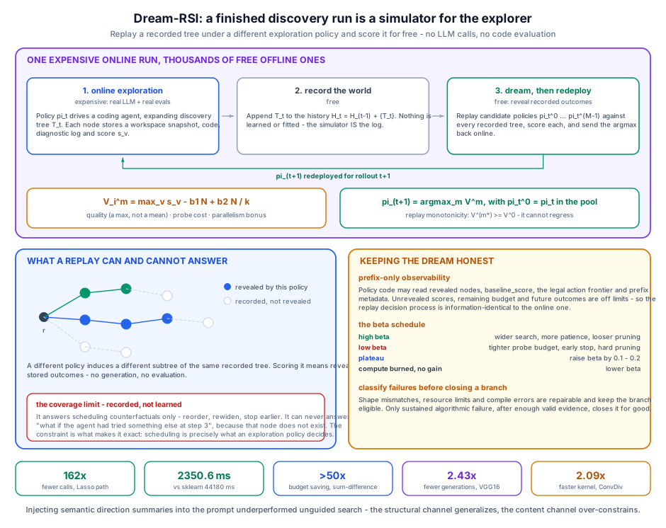
Dream-RSI’s move is to notice that you already ran them. A completed discovery run leaves behind a tree with every node’s code, log, and score recorded. A different exploration policy, replayed against that tree, induces a different subtree, and scoring it requires only revealing the outcomes that are already stored. No generation, no evaluation, no GPU. One expensive online run becomes thousands of free offline policy evaluations.
1. The Analogy, and Where It Diverges
The framing is model-based RL. Dreamer and its relatives learn a world model, then train the policy inside it, so most policy improvement costs simulator steps rather than environment steps.
Dream-RSI does the same thing with one difference that matters: the world model is not learned, it is recorded. There is no model error, no compounding rollout divergence, no dreaming about states that cannot happen. Every node the replay reveals is a real code artifact that really scored what it says it scored.
The price is coverage. A learned world model can be queried anywhere; a recorded tree can only answer questions about branches that were actually taken. You cannot ask “what if the agent had tried a completely different approach at step 3”; that node does not exist. The replay simulator answers scheduling counterfactuals (different order, different width, different stopping point over the same node set) and nothing else.
That constraint is what makes it work. Scheduling is exactly what an exploration policy decides.
2. Discovery Trees and What a Policy Can Do With One
During online execution the coding agent builds a discovery tree $T$ rooted at $r$, the initial workspace. Each non-root node $v$ has a primary parent whose workspace state and accumulated context it inherits, and stores the candidate’s code, diagnostic log, and scalar score $s_v$.
The policy sees the currently revealed tree $T^{obs}$ and picks nodes to expand:
\[A(T) = \{r\} \cup \{v \in T : v \text{ is a leaf}\}\]Either start a fresh branch from the root, or extend a current frontier. With $W$ parallel worker slots, the policy commits to a batch:
\[A(T; W) = \{C \subseteq A(T) : |C| \le W\}\]So an exploration policy is a function from revealed tree to node batch. Everything it controls (width, depth, order, restarts, stopping) lives in that one choice.
Online rollout. At round $k$, policy $\pi_t$ selects $C_k^t \in A(T_t^k; W)$; each chosen node gets a worker, which generates a new stochastic child:
\[T_t^{k+1} = T_t^k \cup \bigcup_{v \in C_k^t} \text{Child}(v)\]After up to $K_1$ rounds the tree is appended to the history: $\mathcal{H}_t = \mathcal{H}_{t-1} \cup \{T_t\}$.
Offline replay. Now the same interface, deterministic. Policy version $\pi_t^m$ replays against a fixed $T_i \in \mathcal{H}_t$, starting from $T_i^{m,0} = \{r\}$. Selecting a batch reveals recorded children:
\[T_i^{m,k+1} = T_i^{m,k} \cup \bigcup_{v \in C_i^{m,k}} \text{Child}(v; T_i, T_i^{m,k})\]with two reveal rules:
- $v \ne r$: reveal $v$’s unique unrevealed recorded child.
- $v = r$: reveal the earliest-created unrevealed child of the root, i.e. open the next branch in creation order.
Replay ends when the policy selects $C = \emptyset$, hits the round limit $K_2$, or exhausts $T_i$.
The root rule is doing quiet work. It imposes a canonical order on “start a new branch,” which is what lets a policy that fans out differently than the original still be scored against the same recorded material.
3. Scoring a Dreamed Trajectory
Replaying policy $m$ on world $i$ reveals $N_i^m = |T_i^{m,k_{m,\star}^i}| - 1$ non-root nodes over $k_{m,\star}^i$ rounds. Those are the simulated generate-and-evaluate attempts. The score:
\[V_i^m = \underbrace{\max_{v \in T_i^{m,k_{m,\star}^i}} s_v}_{\text{quality}} \;-\; \underbrace{\beta_1 N_i^m}_{\text{cost}} \;+\; \underbrace{\beta_2 \frac{N_i^m}{\max\{1, k_{m,\star}^i\}}}_{\text{parallelism}}\]Three terms, and the third is the one that is easy to miss.
Quality is the best score found: discovery is a max, not a mean. Finding one excellent solution and forty bad ones is a success.
Cost penalizes total attempts, which is what prevents the trivial optimum of revealing the entire tree.
Parallelism rewards $N/k$, the average attempts per decision round. Without it, quality-minus-cost is indifferent between 40 attempts in 40 sequential rounds and 40 attempts in 5 wide batches. Those cost the same LLM budget and wildly different wall clock. The third term is what makes the policy schedule for a real machine rather than a token counter.
Averaged over all $t$ recorded worlds:
\[V^m = \frac{1}{t}\sum_{i=1}^{t} V_i^m\]3.1 Improvement, and the guarantee that comes with it
An LLM policy-development agent reads the replay traces, diagnoses failure modes, and writes $M$ candidate revisions $\pi_t^0, \dots, \pi_t^{M-1}$, where $\pi_t^0 = \pi_t$ is the incumbent. Selection is greedy:
\[\pi_{t+1} = \pi_t^{m^\star}, \qquad m^\star \in \arg\max_{m} V^m\]Because the incumbent is in the candidate pool,
\[V^{m^\star} \ge V^0\]Replay monotonicity: the redeployed policy is never worse than its predecessor on the historical replay set. The hedge matters: this is a guarantee about $\mathcal{H}_t$, not about the next online run, and the two can diverge when the next problem differs from every recorded one. But it is the same structural safety net as the sorted acceptance test in greedy model soups: include the incumbent, select by argmax, and the procedure cannot regress on the data it selected from. It turns self-improvement from a gamble into a ratchet.
4. Keeping the Dream Honest
Offline evaluation against recorded outcomes has an obvious way to cheat: look at the scores before deciding which nodes to reveal. A policy that peeks scores perfectly in replay and is useless online.
Prefix-only observability. Policy code may read only revealed nodes, the baseline_score, the legal action frontier, and prefix structural metadata. Unrevealed scores, remaining budget, and future trace outcomes are off limits. This makes the replay decision process genuinely match the online one: the policy has the same information in both, so a replay win means something.
The $\beta$ schedule. The exploration/exploitation dial. High $\beta$: wider search, more patience per branch, looser pruning. Low $\beta$: tighter probe budget, early stopping on stagnating branches, aggressive pruning of weak directions. (The objective in §3 carries two coefficients, $\beta_1$ and $\beta_2$, while the tuning discussion talks about a single scalar $\beta$; I read the latter as the exploration knob the policy agent actually turns, with the pair moving together, but the source is not explicit about the relationship.) Offline, $\beta$ is swept as a grid, free, since replay is free. Online, it is adjusted by observation: plateau → raise $\beta$ by 0.1–0.2 to buy exploration; compute burned without quality gains → lower $\beta$.
Failure classification before closure. Deciding to abandon a branch requires knowing why it failed. The controller reconstructs the full prefix trajectory and classifies:
- Repairable: shape mismatches, resource limits, naming bugs, compilation errors. The branch stays eligible; these say nothing about whether the approach is sound.
- Hard: sustained algorithmic failure after enough valid evidence. Close it permanently.
Conflating the two is how a search kills a good idea over a typo, and it is the kind of judgment a fixed heuristic has no way to express.
5. Results
Eight tasks across three domains.
| Domain | Task | Result | Efficiency |
|---|---|---|---|
| Algorithm engineering | Lasso regularization path (17 synthetic, 6 held-out) | 2350.6 ms avg vs sklearn 44180 ms, glmnet 13767 ms, SimpleTES 3804 ms | $162\times$ fewer calls than SimpleTES; $1.7\times$ fewer than fixed exploration |
| Mathematical optimization | Sum–difference problem | 1.145427 vs SimpleTES 1.143975 | $>50\times$ budget saving, $<1$k vs 51,200 generations |
| Mathematical optimization | Circle packing, $n \in \{26, 32\}$ | 2.635983, matching SOTA | $<1$k generations |
| GPU kernels | KernelBench VGG16, LayerNorm | Reaches SOTA kernel speed | $2.43\times$ fewer generations (VGG16), $1.79\times$ (LayerNorm) |
| GPU kernels | KernelBench ConvDiv, ConvMax | $2.09\times$ / $1.44\times$ faster kernels | Same budget |
Two distinct wins are stacked here and they are worth separating. On VGG16 and LayerNorm the discovered artifact is equally good and reached with 2–2.4× less search. On ConvDiv and ConvMax the budget is held fixed and the artifact is better. Same mechanism, a better exploration policy, cashed out in whichever currency the benchmark measures.
The Lasso numbers are the headline: 18.8× faster than sklearn and 5.9× faster than glmnet, found with 162× fewer LLM calls than the baseline discovery system. The compute-efficiency claim and the quality claim are not in tension, which is the point of the whole paper.
5.1 What it found
The discovered Lasso solver is C++/OpenMP and combines three ideas:
Workload-aware Cauchy–Schwarz KKT pruning. Compute an exact feature gradient only when the analytical bound cannot certify the feature is inactive:
\[\text{Bound}_j = \left|\nabla F_j^{\text{ref}}\right| + s_j \cdot d > \text{KKT}_{\text{bound}}\]double diff = r_curr_ptr[k] - r_ref_ptr[k];
d2 += diff * diff;
double d = std::sqrt(d2);
for (int i = 0; i < unscreened_size; ++i) {
int j = unscreened_ptr[i];
double bound = std::abs(grad_ref_ptr[j]) + s_ptr[j] * d;
if (bound > KKT_bound) {
to_compute.push_back(j); // only here do we pay for an exact gradient
}
}
Disjoint partition tracking. Active, screened, and unscreened feature sets maintained as array partitions with $O(1)$ swap-deletion, so set membership costs nothing per iteration.
Fused FTPP and hardware alignment. Transposition, precomputation, and 64-byte aligned padding folded into a single cache-blocked OpenMP SIMD pass.
Note the flavor: safe screening with a Cauchy–Schwarz bound is classical Lasso literature, and the 64-byte alignment and cache blocking are classical performance engineering. The discovery is the fusion, and the composition of a numerical-analysis idea with a memory-layout idea in one pass is exactly what tends to fall between two specialists. The same pattern shows up in the agentic kernel work in CUDA Agent and Cake.
5.2 Two findings I did not expect
Prompt-level guidance made things worse. Injecting explicit high-level semantic direction summaries into the agent’s prompts consistently underperformed unguided exploration. Telling the agent what to try collapses search diversity; letting a replay-optimized policy shape the structure of the search preserves it.
This is a real distinction and an actionable one. Meta-level improvement can act on content (what to attempt) or on structure (how to schedule attempts). The content channel is the intuitive one and it over-constrains. The structural channel is the one that generalizes: it never asserts anything about the problem domain, so it cannot be wrong about it.
The learned policy allocates effort non-monotonically. It drops from 110 attempt calls to 50 when progress is steady, and widens branching automatically on plateaus. Nobody specified that schedule; it fell out of optimizing $V$ against recorded trees. It is also the behavior a good engineer exhibits (push hard when stuck, coast when the current direction is working), and it is precisely what a fixed heuristic cannot do.
That “spend more where you are stuck, less where you are already winning” shape is the same reallocation logic that Never Give Up applies to RL rollout budget: the fixed-budget default is a resource allocation nobody chose, and adapting it online is where the compute savings live.
6. Takeaways
Discovery logs are an asset, not an archive. The reframe is the contribution. Most agent systems write their traces to disk, use them as prompt context at best, and treat them as exhaust. Dream-RSI treats a completed run as a simulator for the meta-level, and gets thousands of zero-cost policy evaluations out of a run that was going to happen anyway. If you operate any long-horizon search agent, you are probably sitting on this and not using it.
Recorded beats learned when scheduling is the question. A recorded tree cannot answer content counterfactuals, but it answers scheduling counterfactuals exactly, with no model error. Matching the simulator’s fidelity to the decision you are optimizing is a better trade than a general world model here; the contrast with a learned model like ECHO is instructive.
Decouple the orchestrator from the agent. The exploration policy and the coding agent are separate objects with separate improvement loops, which is why the policy can be optimized off-policy at all. The self-improvement and harness-evolution literature keeps landing on the same structural point: the thing you can safely improve is the scaffolding, not the model, and this is the cleanest formalization of that I have seen: the policy is code, the objective is measurable offline, and the update has a monotonicity guarantee.
Include the incumbent. $\pi_t^0 = \pi_t$ in the candidate pool is one line and it converts an open-ended self-modification loop into something that provably cannot regress on its own history. Every self-improving system should have this property and most do not.
Prefix-only observability is the load-bearing constraint. Without it the whole thing is a benchmark-gaming exercise. It is worth noting how much care the design puts into making the offline decision process information-identical to the online one. That discipline, not the replay idea, is what makes the offline scores predictive.
The broader point, and the one that connects to Jeff Dean’s framing of self-improving systems: the bottleneck in long-horizon discovery is no longer raw model capability. It is meta-level orchestration, and orchestration, unlike model weights, is cheap to evaluate offline if you kept your logs.