Averaging the Sweep: Ensemble Accuracy at Single-Model Inference Cost
Reading notes on:
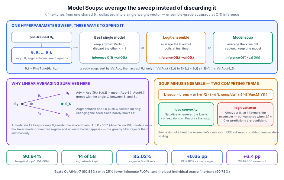
The standard fine-tuning pipeline has a step in it that nobody defends, because nobody looks at it. You sweep hyperparameters (learning rate, augmentation, weight decay, epochs, seed), you get $k$ fine-tuned checkpoints, you score them on a validation set, you keep $\theta_j = \arg\max_i \text{ValAcc}(\theta_i)$, and you delete the other $k-1$. All that compute, discarded on the grounds that you can only ship one model.
The alternative everybody knows about is ensembling the logits, which works and which nobody does at scale, because it multiplies inference latency and memory by $k$. So the field settled into a quiet trade: ensemble accuracy is real but unaffordable, therefore pick one.
Model soups break the trade. Because models fine-tuned from a common pre-trained initialization $\theta_0$ stay inside a shared low-error basin, you can average their weights rather than their outputs:
\[\theta_S = \frac{1}{|S|} \sum_{i \in S} \theta_i, \qquad S \subseteq \{1, \dots, k\}\]The result is one parameter vector. One forward pass. $O(1)$ inference compute and memory, identical to the single model you were going to ship anyway, with accuracy and distribution-shift robustness that beats it, and in the headline result beats the ensemble too.
1. Three Recipes
Fine-tuning under hyperparameter configuration $h_i$ produces $\theta_i = \text{FineTune}(\theta_0, h_i) \in \mathbb{R}^d$. The question is only which subset $S$ to average and with what weights.
| Method | Parameter vector | Inference cost | Validation cost |
|---|---|---|---|
| Best single model | $\theta_{\text{best}} = \arg\max_{\theta_i} \text{ValAcc}(\theta_i)$ | $O(1)$ | $O(k)$ |
| Logit ensemble | $f_{\text{ens}}(x) = \frac{1}{k}\sum_{i=1}^k f(x, \theta_i)$ | $O(k)$ | $O(k)$ |
| Uniform soup | $\theta_S = \frac{1}{k}\sum_{i=1}^k \theta_i$ | $O(1)$ | $O(1)$ |
| Greedy soup | $\theta_S$ via Algorithm 1 | $O(1)$ | $O(k)$ |
| Learned soup | $\theta_S = \sum_{i=1}^k \alpha_i \theta_i$ | $O(1)$ | gradient optimization |
1.1 Uniform soup
Average everything, no filtering: $S = \lbrace 1, \dots, k \rbrace$. This works when every candidate is uniformly decent, and fails badly otherwise: a single run that diverged under an over-large learning rate drags the whole average down. That fragility is the entire motivation for the next recipe.
1.2 Greedy soup
Algorithm 1 builds $S$ sequentially, admitting a candidate only if it does not hurt held-out accuracy:
- Sort candidates by decreasing validation accuracy: $\text{ValAcc}(\theta_1) \ge \text{ValAcc}(\theta_2) \ge \dots \ge \text{ValAcc}(\theta_k)$.
- Initialize $S \leftarrow \lbrace 1 \rbrace$, $\theta_S \leftarrow \theta_1$.
- For $i = 2, \dots, k$:
- Form the candidate average $\displaystyle \theta_{\text{cand}} = \frac{1}{\lvert S\rvert + 1}\Big(\sum_{j \in S}\theta_j + \theta_i\Big)$.
- If $\text{ValAcc}(\theta_{\text{cand}}) \ge \text{ValAcc}(\theta_S)$, set $S \leftarrow S \cup \lbrace i \rbrace$ and $\theta_S \leftarrow \theta_{\text{cand}}$.
- Return $\theta_S$.
The sorting step is what makes this safe. Since $\theta_1$ is the best individual model and nothing is admitted that lowers the score, greedy soup is guaranteed to be at least as good as the best single model on $D_{\text{val}}$. It is a strict improvement over the baseline procedure it replaces, not a gamble, which is the property that makes it worth putting in a pipeline by default.
It is also self-repairing in the way uniform soup is not: a divergent run simply fails the acceptance test and never enters $S$.
1.3 Learned soup
Drop the greedy heuristic and optimize the mixing coefficients $\boldsymbol{\alpha} \in \mathbb{R}^k$ and a temperature $\beta$ directly on the validation set:
\[\min_{\boldsymbol{\alpha}, \beta} \sum_{j=1}^{n_{\text{val}}} \ell\left(\beta \cdot f\Big(x_j, \sum_{i=1}^k \alpha_i \theta_i\Big), y_j\right)\]with $\alpha_i = \exp(\gamma_i) / \sum_m \exp(\gamma_m)$ to keep the mixture positive and bounded. A layer-wise variant learns separate $\boldsymbol{\alpha}^{(l)}$ per layer. The cost is that you need all $k$ models resident to compute a gradient, which greedy soup does not.
2. Why Linear Averaging Is Legal Here
The obvious objection is that averaging weights of two networks should destroy them. For networks trained from random initializations it does exactly that: their solutions sit in distinct basins separated by high error barriers, and the midpoint is near-random.
The pre-trained initialization is what changes the picture. Fine-tuning from a shared $\theta_0$ keeps the runs in one basin, linearly mode-connected, and the segment between any two of them stays low-loss.
2.1 The angle predicts the gain
Define the trajectory vectors $\delta_1 = \theta_1 - \theta_0$ and $\delta_2 = \theta_2 - \theta_0$, and the angle between them:
\[\cos\phi = \frac{\langle \theta_1 - \theta_0,\, \theta_2 - \theta_0\rangle}{\|\theta_1 - \theta_0\|\,\|\theta_2 - \theta_0\|}\]The interpolation advantage
\[\text{Adv}(\theta_1, \theta_2) = \text{Acc}\left(\frac{\theta_1 + \theta_2}{2}\right) - \frac{\text{Acc}(\theta_1) + \text{Acc}(\theta_2)}{2}\]correlates strongly and positively with $\phi$. Trajectories that head off in near-orthogonal directions ($\phi \to 90^\circ$) produce complementary error patterns, and averaging them cancels errors rather than averaging them.
This is the practical lesson buried in the geometry, and it is an actionable one: vary the things that move the trajectory, not the things that don’t. Data augmentation, loss function, and learning rate push $\phi$ toward orthogonality. Re-running with a different random seed barely moves it, which is why seed-only sweeps make disappointing soup.
2.2 Where the basin ends
The basin is not unbounded. Push the learning rate too high ($\text{LR} \ge 10^{-4}$ for AdamW on ViT is the paper’s marker) and runs exit the linear mode connectivity regime. Average across an error barrier and accuracy collapses. Greedy soup handles this without special-casing: such a model fails the acceptance test and is dropped.
3. Soup vs. Ensemble, Derived
Weight averaging and logit averaging are different operations that happen to agree sometimes. The paper makes “sometimes” precise. Let $\theta_\alpha = (1-\alpha)\theta_0 + \alpha\theta_1$, with $f^{\text{soup}}_\alpha(x) = f(x; \theta_\alpha)$ and $f^{\text{ens}}_\alpha(x) = (1-\alpha)f(x;\theta_0) + \alpha f(x;\theta_1)$.
Step 1: an exact integral for the logit gap
With $\delta = \theta_1 - \theta_0$, two applications of the fundamental theorem of calculus give an exact expression:
\[f^{\text{ens}}_\alpha(x) - f^{\text{soup}}_\alpha(x) = \int_0^1 \left(\delta^T \nabla^2_\theta f(x; \theta_\tau)\,\delta\right) w_\alpha(\tau)\, d\tau\]where $w_\alpha(\tau) = \min\lbrace (1-\alpha)\tau,\ \alpha(1-\tau) \rbrace$ and $\int_0^1 w_\alpha(\tau)\,d\tau = \frac{\alpha(1-\alpha)}{2}$.
The gap is therefore entirely a curvature effect. If the logits were linear in $\theta$ along the segment, the Hessian would vanish and soup and ensemble would be identical. Assuming the logits are approximately quadratic along $\theta_\tau$, so $\nabla^2_\theta f(x;\theta_\tau) \approx \nabla^2_\theta f(x;\theta_\alpha)$:
\[f^{\text{ens}}_\alpha(x) - f^{\text{soup}}_\alpha(x) \approx \frac{\alpha(1-\alpha)}{2}\,\delta^T \nabla^2_\theta f(x;\theta_\alpha)\,\delta\]Step 2: pushing through the cross-entropy
For $\ell(f, y) = \log\big(\sum_{y’}\exp(f_{y’} - f_y)\big)$ we have $\nabla_f \ell = p_{\text{sftmx}}(f) - e_{(y)}$ and $\nabla^2_f \ell = \text{diag}(p_{\text{sftmx}}(f)) - p_{\text{sftmx}}(f)p_{\text{sftmx}}(f)^T$. A first-order expansion of the ensemble loss around the soup logits gives
\[\ell(f^{\text{ens}}_\alpha; y) - \ell(f^{\text{soup}}_\alpha; y) \approx \left[\nabla_f \ell(f^{\text{ens}}_\alpha; y)\right]^T \left(f^{\text{ens}}_\alpha - f^{\text{soup}}_\alpha\right)\]and the chain rule relates the parameter-space Hessian of the loss to logit gradients and logit Hessians:
\[\delta^T \nabla^2_\theta \ell(f(x;\theta_\alpha); y)\,\delta = \left[\delta^T \nabla_\theta f\right]^T \nabla^2_f \ell(f;y) \left[\delta^T \nabla_\theta f\right] + \left[\nabla_f \ell(f;y)\right]^T\!\left(\delta^T \nabla^2_\theta f(x;\theta_\alpha)\,\delta\right)\]Approximating $\delta^T \nabla_\theta f(x;\theta_\alpha) \approx f(x;\theta_1) - f(x;\theta_0) = \Delta f(x)$, the first term becomes a variance under the model’s own predictive distribution:
\[\left[\delta^T \nabla_\theta f\right]^T \nabla^2_f \ell(f;y) \left[\delta^T \nabla_\theta f\right] = \text{Var}_{Y \sim p_{\text{sftmx}}(f^{\text{soup}}_\alpha(x))}\left[\Delta f_Y(x)\right]\]Step 3: the master formula
Folding in an inverse temperature $\beta$ for calibration:
\[\mathcal{L}^{\text{soup}}_\alpha - \mathcal{L}^{\text{ens}}_\alpha \approx \frac{\alpha(1-\alpha)}{2}\left(-\frac{d^2}{d\alpha^2}\mathcal{L}^{\text{soup}}_\alpha + \beta^2\,\mathbb{E}_{x,y}\left[\text{Var}_{Y \sim p_{\text{sftmx}}(\beta f(x;\theta_\alpha))}\left[\Delta f_Y(x)\right]\right]\right)\]Two forces, pulling opposite ways:
- Loss convexity, $-\frac{d^2}{d\alpha^2}\mathcal{L}^{\text{soup}}_\alpha$. If the soup loss is strictly convex along the interpolation path, this is negative and favours the soup over either endpoint. This is the term that makes averaging a win rather than a compromise.
- Logit variance, $\beta^2\mathbb{E}[\text{Var}(\Delta f_Y)]$. Non-negative always, so it favours the ensemble. But it shrinks to nothing in two regimes that fine-tuned models routinely occupy: when the models are close in logit space ($\Delta f(x) \approx 0$), and when predictions are confident, so $p_{\text{sftmx}}(\beta f)$ approaches a point mass and the variance under it collapses.
That is the whole story of why soups are competitive with ensembles at the frontier and not merely a cheap approximation of them. High-accuracy fine-tunes of a shared backbone are confident and mutually close, precisely the corner where term 2 vanishes and term 1 does not.
4. What the Numbers Say
4.1 ImageNet with ViT-G/14
Greedy soup over 58 fine-tuned ViT-G/14 models (JFT-3B pre-trained) selected 14 ingredients and set a new state of the art.
| Model / method | Top-1 | IN-V2 | IN-R | IN-Sketch | ObjectNet | IN-A | Avg shifts |
|---|---|---|---|---|---|---|---|
| ViT-G/14 baseline | 90.47% | 83.39% | 94.38% | 72.37% | 71.16% | 89.00% | 82.06% |
| Best individual (val) | 90.72% | 83.76% | 95.04% | 73.16% | 78.20% | 91.75% | 84.38% |
| Best individual (oracle) | 90.78% | 84.31% | 95.04% | 73.73% | 79.03% | 92.16% | 84.68% |
| Greedy ensemble | 90.93% | 84.14% | 94.85% | 73.07% | 77.87% | 91.69% | 84.33% |
| Greedy soup | 90.94% | 84.22% | 95.46% | 74.23% | 78.52% | 92.67% | 85.02% |
Two things stand out. The soup edges past CoAtNet-7 (90.88%) while using 25% fewer inference FLOPs, and it beats the greedy ensemble (90.93%) that costs $k\times$ more to serve. And the robustness gap is wider than the in-distribution one: +0.16 pp over the oracle single model on ImageNet top-1, but +0.34 pp on the shift average, and +0.69 pp on shifts over the greedy ensemble, which it only edges by 0.01 pp in distribution. The largest single-benchmark gains over the oracle are ImageNet-Sketch (+0.50) and ImageNet-A (+0.51).
One detail worth reading carefully: the oracle row is the only one whose cells do not average to its own “Avg shifts” entry: the five values mean to 84.85%, not 84.68%. That is not a typo. The other rows are each a single model, so their cells average out exactly. The oracle row is not one model: each cell is the best individual model on that benchmark, so the cells can come from different checkpoints, and the mean of per-column maxima is always at least the maximum of per-row means. The 84.68% is the best single model as measured on the shift average, which is the honest baseline to compare a soup against.
4.2 CLIP and ALIGN
- CLIP ViT-B/32, 72 models from random hyperparameter search: greedy soup reaches 81.03% on ImageNet against 80.38% for the best single model (+0.65 pp), and 50.75% on the five distribution shifts against 47.83% (+2.92 pp). Note the ratio: the robustness gain is over four times the in-distribution gain.
- ALIGN EfficientNet-L2, 12 models from grid search: +0.5 pp on ImageNet over the best individual fine-tune.
4.3 NLP: BERT and T5 on GLUE
The technique is not vision-specific.
- T5-base: MRPC $91.8 \to 92.4$, RTE $78.3 \to 79.1$, CoLA $58.8 \to 60.2$, SST-2 $94.6 \to 94.7$.
- BERT-base: RTE $61.0 \to 61.7$, SST-2 $92.5 \to 93.0$.
The pattern is consistent with the geometry argument: the biggest gains land on the small, high-variance tasks (RTE, CoLA, MRPC) where individual fine-tuning runs scatter most, and the smallest on the large, saturated one (SST-2).
4.4 Cross-dataset soups
The most surprising result. Take a zero-shot CLIP backbone, fine-tune it independently on six datasets (ImageNet, CIFAR-10, Food-101, SUN397, Stanford Cars, DTD), average the backbone weights while keeping the zero-shot text heads, and evaluate zero-shot on a dataset that was in none of the runs: CIFAR-100 improves by +6.4 pp.
Here the ingredients were not even trained on the same objective. The basin argument survives changing the task, not just the hyperparameters.
5. Engineering Notes
- EMA interacts with souping, and not in the obvious direction. When fine-tuning very large models (ViT-G/14, BASIC-L), a low EMA decay ($\beta = 0.999$) produces better soup ingredients than a high one, even when the high-EMA runs score better individually. Selecting ingredients by individual accuracy is the wrong objective; you want ingredients that combine well.
- Soups do not fix calibration. Unlike logit ensembling, weight averaging does not automatically improve Expected Calibration Error. If you need calibrated probabilities, apply post-hoc temperature scaling to the soup. This is worth flagging in any pipeline where the model’s confidence feeds a downstream decision. See the stage-by-stage view in Metrics and Benchmarks Across LLM Training Stage.
- Learning rate is the main failure mode. Beyond roughly $10^{-4}$ (AdamW on ViT) you are averaging across a barrier. Algorithm 1 filters these automatically, which is another reason to prefer greedy over uniform.
- Tied embeddings will bite you. Many Transformers tie the input embedding to the output classifier. Averaging with in-place updates corrupts shared-pointer memory. Copy before you accumulate.
- Composes with SWA and SAM. Gains from model soups are additive with Stochastic Weight Averaging and Sharpness-Aware Minimization; all three are attacking flatness from different angles, and none of them subsume the others.
6. Takeaways
Stop deleting your sweep. If you fine-tune 20–50 models during hyperparameter optimization, running Algorithm 1 over the checkpoints costs $O(k)$ validation passes (which you already paid for, since you had to score them to pick a winner) and is provably no worse than the model you would have shipped.
The deployment cost is zero. Not “small.” Zero. One weight vector, one forward pass, no added memory, no added latency. This is the property that separates soups from every other accuracy-for-compute trade in the fine-tuning literature.
Diversify along the axes that move the trajectory. Augmentation strategy, loss function, and learning rate widen $\phi$; seeds barely do. If you are designing a sweep with souping in mind, that changes what you sweep over.
The scope condition is a shared initialization. Everything here rests on all ingredients descending from one $\theta_0$ and staying in its basin. That is a real limit: it is why you cannot soup two independently pre-trained models, and why merging across genuinely different models needs a different mechanism entirely: behavioural transfer, as in Breaking the Tokenizer Barrier, rather than parameter arithmetic.
The broader framing I keep coming back to: fine-tuning produces a distribution over solutions, and the standard pipeline treats that distribution as noise to be filtered down to a single sample. Souping treats it as signal. That is the same move as the shift from picking checkpoints to reasoning about what each post-training stage does to the model’s distribution (see The Distributional Lens of Post-Training), and it rhymes with why flatness-seeking optimizers work at all, discussed in SOAP, Muon, and Beyond.