Never Give Up: Fixing the Matthew Effect in LLM RL
Reading notes on:
- Learning to Solve Hard Problems in RL for LLMs by Never Giving Up
- Learning to Solve Hard Problems in RL for LLMs by Never Giving Up (arXiv:2609.13443)
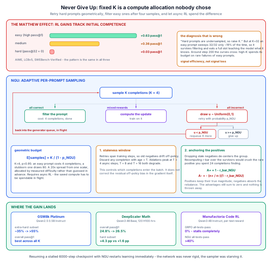
RL post-training works, and the aggregate numbers hide where it works. Break the gains down by initial difficulty and a uniform pattern appears across math, code completion, and agentic coding:
| Initial competence | RL gain (pass@1) |
|---|---|
| High (easy problems) | +0.63 |
| Medium | +0.36 |
| Low / zero (hard problems) | +0.03 |
Problems the model already mostly solves get much better. Problems it cannot solve at all stay unsolved. On AIME, prompts with initial $\text{pass}@32 = 0$ finish near $0\%$; prompts above 30% initial accuracy improve dramatically. This is the Matthew effect, the rich get richer, and it means your RL run is largely polishing the part of the distribution you were least worried about.
The obvious diagnosis is that hard problems are undersampled, so sample them more. That diagnosis is wrong in an interesting way, and getting it right is what makes NGU a 20-line change rather than a new algorithm.
1. Signal Loss Is Not the Problem
GRPO samples $K$ completions for each of $N$ prompts. For prompt $x$ with binary rewards $r_i \in \{0,1\}$:
\[\bar{r} = \frac{1}{K}\sum_{j=1}^{K} r_j, \qquad A_i = r_i - \bar{r}\]The zero-gradient condition is what drives everything downstream: if all $K$ completions are correct, or all are incorrect, then $A_i = 0$ for every $i$ and the prompt contributes nothing. Such prompts get filtered.
So the intuitive fix for hard problems is to raise $K$: more samples, better odds of stumbling onto a rare correct completion, gradient signal where there was none. That is treating the problem as signal loss: the positives exist but you are not finding them.
1.1 The high-$K$ paradox
Raising $K$ does find more rare positives on hard problems. It also finds more rare negatives on easy problems, and that turns out to dominate.
Consider a prompt the model solves 95% of the time. At $K=4$, the chance of a clean 4/4 sweep is about 81%: the prompt gets filtered out and costs nothing further. At $K=32$, a clean 32/32 sweep happens about 19% of the time. The other 81% of the time, one or two unlucky failures give the prompt a non-zero advantage and it stays in the batch, consuming a full 32-completion slot to teach the model something about a problem it already knows.
The empirical signature: early in training $K=32$ does include more hard problems, but around step 200 the curves cross. By then $K=4$ has purged the easy prompts through aggressive filtering, while $K=32$ is still dragging them along. High-$K$ GRPO ends up spending most of its compute training on noise, and the fraction of the batch that is hard problems goes down even as the absolute count goes up.
So the real problem is signal efficiency, not signal loss. There is plenty of budget; it is going to the wrong prompts. Fixed $K$ is the bug: it forces the same sampling budget on a prompt the model solves 19 times out of 20 and a prompt it has never solved.
2. NGU: Retry Until You Give Up
Make $K$ adaptive, per prompt, online, with one parameter.
- Sample $K$ completions (default $K = 4$).
- All correct? Discard the prompt as easy. Compute saved.
- Mixed rewards? Non-zero advantages exist; compute the GRPO update and train.
- All incorrect? Draw $u \sim \text{Uniform}(0,1)$:
- $u < p_{\text{NGU}}$: push the prompt back into the generator queue for $K$ more completions.
- $u \ge p_{\text{NGU}}$: give up on it.
The per-prompt completion count is now geometric rather than fixed:
\[\mathbb{E}[\text{samples}] = \frac{K}{1 - p_{\text{NGU}}}\]With $K=4$ and $p_{\text{NGU}} = 0.95$: an easy prompt costs 4 completions, a persistently hard one draws 80 in expectation. A 20× spread in budget, allocated by observed difficulty rather than guessed in advance, with a single scalar controlling it.
Two properties worth noticing. The allocation is online: difficulty is measured against the current policy, so a prompt that becomes easy at step 400 stops being expensive at step 400. And the retry is probabilistic rather than bounded, so there is no cap to tune and no prompt that stalls the pipeline forever.
2.1 Why this needs async RL
NGU is not really a sampling change; it is a reallocation change, and reallocation requires that the compute saved on easy prompts be immediately spendable elsewhere. That only works on an asynchronous framework (Async RLHF, PipelineRL) where the generator runs decoupled from the trainer.
Under synchronous RL, filtering an easy prompt in 4 completions just leaves a worker idle until the batch barrier. The generator has to be free to pull the requeued hard prompt into the slot the easy prompt vacated, in flight, without the trainer waiting. The batch composition drifts toward hard problems as a consequence of the generator’s queue discipline, not because anyone reweighted a sampler.
This is the same generator/trainer throughput-matching concern from the other direction: there, keeping both sides busy is the goal; here, an async pipeline is the precondition for an algorithmic idea to work at all.
3. The Two Corrections That Make It Work
Asynchronous retries mean a prompt’s completions now span several training steps. Two problems follow, and both fixes are small.
3.1 Staleness window
Old negative completions were generated by an older policy. Keeping them injects off-policy noise into exactly the gradient you were trying to sharpen. NGU tags each completion with an age and discards any with
\[\text{age}(y_i) > T\]Ablations put the optimum at $T = 4$ async steps; $T = 8$ and $T = 16$ both degrade performance. Narrow window, and the value of an old negative decays fast. (Note what this does not fix: the residual off-policy bias in the gradient itself, which is the drift term that Score Centering targets. The two are complementary: NGU controls which completions enter the batch, SC corrects the gradient given that they did.)
3.2 Anchoring the positives
Here is the subtle part. Say a prompt has been retried five times: 20 completions total, all negative, and then on the sixth attempt one completion is finally correct. The historical group mean is
\[\bar{r}_{\text{NGU}} = \frac{1}{24} \approx 0.042\]computed over all 24 completions. But you only keep the non-stale ones, say 4 of them. If you naively apply $A_i = r_i - \bar{r}_{\text{NGU}}$ to the surviving 4, the advantages no longer sum to zero, and the batch is miscentered.
The obvious repairs are both bad. Recompute $\bar{r}$ over just the survivors and you inflate the apparent solve rate, crushing the advantage on the rare positive you worked 24 completions to find. Downsample the negatives to match the positives and you throw away fresh contrastive signal.
NGU’s answer keeps the positive’s advantage at its true historical value and rescales the negatives to restore the zero sum:
\[A_i^{+} = 1 - \bar{r}_{\text{NGU}}, \qquad A_j^{-} = -\frac{n^{+}}{n^{-}}\left(1 - \bar{r}_{\text{NGU}}\right)\]where $n^{+}$ is the number of positives and $n^{-}$ the number of surviving non-stale negatives. Check the sum:
\[n^{+}\left(1 - \bar{r}_{\text{NGU}}\right) + n^{-}\cdot\left(-\frac{n^{+}}{n^{-}}\left(1 - \bar{r}_{\text{NGU}}\right)\right) = 0\]So the rare positive gets the full gradient magnitude its rarity earns ($1 - \frac{1}{24} \approx 0.96$, not the $1 - \frac{1}{4} = 0.75$ you would get from recomputing over survivors), while the negatives absorb the rebalancing. The name is exact: the positives are anchored, the negatives float.
3.3 The loop
def ngu_sampler_thread(generator, trainer, K, p_NGU, buffer_S, T):
    while trainer.is_running():
        x = generator.get_next_prompt()
        y_new = generator.sample(prompt=x, count=K)
        r_new = [reward_fn(x, y) for y in y_new]
        k_curr = K

        # merge in history if this prompt has been retried before
        if x in buffer_S:
            y_old, r_old, k_old, r_bar_old = buffer_S.pop(x)
            r_bar = (r_bar_old * k_old + mean(r_new) * K) / (k_old + K)
            k_curr += k_old
            y_valid = [y for y in y_old if y.age <= T] + y_new
            r_valid = [r for r, y in zip(r_old, y_old) if y.age <= T] + r_new
        else:
            r_bar = mean(r_new)
            y_valid, r_valid = y_new, r_new

        if all(r == 1 for r in r_valid):
            continue                                  # solved -> filter, save compute
        elif any(r > r_bar for r in r_valid):
            adv = compute_anchored_advantages(r_valid, r_bar)
            trainer.submit_update(x, y_valid, adv)    # gradient exists -> train
        else:
            if random.uniform(0.0, 1.0) < p_NGU:      # all wrong -> retry or quit
                generator.requeue(x)
                buffer_S[x] = (y_valid, r_valid, k_curr, r_bar)
The running mean $\bar{r}$ is accumulated over all historical completions (weighted by count), while y_valid holds only the non-stale ones; that split is precisely what §3.2 needs.
4. Results
| Task | Model | Setup | Finding |
|---|---|---|---|
| GSM8k Platinum | Qwen 2.5 0.5B Instruct | $N{=}64, K{=}4, p_{\text{NGU}}{=}0.95$ | Best pass@1 across all $K$ settings; extra-hard subset rises from $\sim35\%$ to $>55\%$ |
| DeepScaler Math (AIME + BRUMO 2025) | Qwen 3 4B Base | $K{=}16, p_{\text{NGU}}{=}0.875$, 120 H100-hrs | Overall pass@1 $24.8\% \to 26.5\%$; hard subset $+4.3$ pp vs $+1.6$ pp for GRPO |
| Manufactoria Code RL | Qwen 3 4B Instruct | $N{=}32, K{=}16, p_{\text{NGU}}{=}0.95$, per-test reward | GRPO stalls at 0% all-tests-pass; NGU exceeds 40% |
The DeepScaler line is the honest one: overall pass@1 moves 1.7 points, which is respectable and not dramatic. The hard-subset number ($+4.3$ pp versus $+1.6$ pp, nearly $2.7\times$) is where the mechanism shows, and the overall gain is muted because hard problems are a minority of the set. NGU is not a general accuracy improvement; it is a redistribution of where improvement lands, and it does that without regressing easy problems.
Manufactoria is the result that is hard to get any other way. Standard GRPO sits at exactly 0% all-tests-pass: not slow progress, no progress, because the all-tests-pass event never occurs in a $K=16$ group and therefore never generates a gradient. NGU crosses 40%. That is a qualitative difference: a capability that does not exist under one budget policy and does under another, on the same model and the same data.
5. Against the Alternatives
No-positive resampling permanently retires a prompt once it is solved 16/16. This mutates the dataset irreversibly, and models regress on previously-solved easy problems in later epochs. NGU’s filtering is per-step and reversible: a filtered prompt is still in the dataset and gets re-examined next time it comes up.
Fixed prompt curricula (GVM-RAFT, Reinforce-Ada-Est) assign $K$ per prompt from initial model accuracy. This improves hard problems and degrades easy ones, for a simple reason: difficulty is not a static property of a problem, it is a property of a problem and the current policy. A budget set at step 0 is wrong by step 500.
Reinforce-Ada is the closest relative, and the differences are instructive:
| Reinforce-Ada | NGU | |
|---|---|---|
| Target | Signal loss (missing positives) | Signal efficiency (misallocated budget) |
| Retry policy | $p = 1.0$: never gives up, stalls on unsolvable prompts | $p_{\text{NGU}} < 1.0$: bounded in expectation |
| Framework | Synchronous | Asynchronous: saved compute is reusable |
| Negatives | Downsampled to match positives | Kept; advantages rescaled instead |
The $p = 1.0$ difference is the operationally important one. An unsolvable prompt under $p=1$ is an infinite loop holding a worker; under $p = 0.95$ the expected cost is bounded and the worker always comes back.
6. Two Things Ruled Out
It is not a harness artifact. In a novel environment like Manufactoria, early failures are mostly the model not understanding the output format, which masks real competence. The Matthew effect only becomes visible after step 100, once harness adaptation is done. That is worth internalizing when reading early-training curves in any new environment: the first phase measures your prompt format, not the model. It is the same confound that makes harness design a first-class variable.
It is not plasticity loss. Deep RL in robotics has a well-documented failure where networks lose the ability to learn anything new. The obvious hypothesis for a model stalled at 0% for thousands of steps is that it has gone rigid. The paper tests it directly: resume from a stagnant 6000-step checkpoint with NGU and learning restarts immediately. The network was never broken. The sampling policy was starving it of gradient, and swapping the sampling policy revives the same weights.
That is a clean experiment and it shifts the conclusion from “the model cannot learn this” to “you never gave it a gradient.”
7. Practical Notes
- $K = 4$ or $K = 16$ as the initial group size. Not 1.
- $p_{\text{NGU}} \in [0.75, 0.95]$. Higher means more persistence on hard prompts.
- $T = 4$ async steps for the staleness window.
- Do not set $K=1$ and lean entirely on $p_{\text{NGU}}$. It produces long generation queues, completions go severely off-policy, and stability degrades. You need enough completions in the first pass to make the all-correct/all-incorrect/mixed decision meaningfully.
- Needs a mixed-difficulty dataset. NGU’s budget for hard prompts is funded by early-filtering easy ones. On a set of uniformly extra-hard prompts (0% initial solve rate) there is nothing to save, and you get higher staleness with no compensating gain.
8. Takeaways
Fixed $K$ is a resource allocation policy nobody chose. It is in every GRPO implementation because it is the simplest thing that types correctly, and it commits identical sampling budget to a problem the model always solves and one it never does. Once you see it as an allocation decision, making it adaptive is obvious, and the fact that one scalar $p_{\text{NGU}}$ buys a 20× budget spread means the lever was cheap the whole time.
The framework enables the algorithm. NGU on synchronous RL is close to pointless: filtering early just idles a worker. On async RL the same rule reallocates in flight. This is one of the clearer cases where a systems property is not an implementation detail of an algorithm but a precondition for it.
Difficulty is a property of the policy, not the dataset. This is the argument against every static curriculum, and it is why online adaptation beats upfront $K$ assignment even when the upfront assignment uses good difficulty estimates.
“The model can’t do this” often means “the model never got a gradient for this.” The stagnant-checkpoint revival is the result I would keep. Before concluding a capability is out of reach, check whether your sampling regime ever produced a non-zero advantage for it.
It pairs with the pre-RL picture. The SFT-to-RL prediction work argues that RL mostly compresses Pass@$k$ mass into Pass@1, which makes the pre-RL Pass@64 ceiling the thing to measure. NGU is the operational counterpart: the way you actually reach the tail of that distribution is to keep sampling the prompts where the mass is thin, and stop sampling the ones where it is already concentrated.