When High SFT Scores Mislead: Predicting Post-RL Performance Before You Run RL
Reading notes on:
The standard reasoning-model pipeline is two stages: supervised fine-tuning, then RL with verifiable rewards. In most organizations those stages are two different teams with two different on-calls, and the interface between them is a number. The SFT team produces checkpoints, ranks them by benchmark Pass@1, hands over the winner, and the RL team takes it from there.
That handoff encodes an assumption nobody writes down: the SFT checkpoint that scores best is the one that will RL best. This paper (ICLR 2026, backed by over a million A100-hours across hundreds of models up to 12B) measures the assumption and finds it is close to worthless. Post-SFT Pass@1 explains 43% of the variance in post-RL outcomes ($R^2 = 0.43$). Worse than uninformative in places: in the failure regimes the correlation goes negative.
The fix is not exotic. Two metrics you can compute on the SFT checkpoint without touching an RL cluster, held-out validation loss $\mathcal{L}_{\text{val}}$ and Pass@64, roughly double $R^2$ and lift rank correlation by up to 50 points.
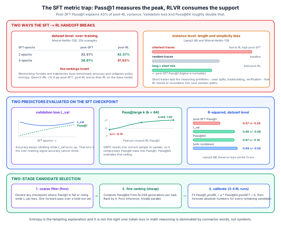
1. Two Ways the Handoff Breaks
The failure is not random noise around a good trend. It is two specific, reproducible mechanisms, one at the dataset level and one at the instance level.
1.1 Dataset level: over-training buys Pass@1 and sells exploration
Train SFT longer on a fixed dataset and post-SFT accuracy goes up. It goes up because the model memorizes formatting conventions and reasoning trajectories, which is exactly what the benchmark measures, and exactly what destroys the thing RL needs.
The cleanest demonstration, on Mistral-NeMo-12B with 25k examples:
| SFT epochs | Post-SFT avg (7 benchmarks) | Post-RL avg |
|---|---|---|
| 2 epochs | 32.51% | 42.57% |
| 4 epochs | 36.61% | 41.63% |
The rankings invert. Four epochs wins the handoff metric by 4.1 points and loses the thing you actually care about by 0.94. Any team selecting on post-SFT score picks the wrong checkpoint, confidently.
Qwen3-4B-base is the sharper version. Post-SFT accuracy climbs from 25.33% to 38.09% over 10k SFT steps (a 12.8-point gain, the kind of curve that gets a checkpoint promoted), and the resulting post-RL performance is worse than running RL on the base model directly. The entire SFT stage was net-negative, and every metric visible at the handoff said it was working.
The mechanism: over-training collapses policy entropy. RLVR needs the policy to still be capable of producing outputs it does not currently favor, because that is where the improvement comes from. A memorized policy has nowhere to explore to.
1.2 Instance level: short traces are easy to learn and bad to learn from
Data-selection heuristics reward short, clean reasoning chains: they converge fast, they produce high post-SFT Pass@1, they look like good data. Training Llama3-8B or Mistral-NeMo-12B on the shortest SFT examples hits strong post-SFT metrics quickly, and then underperforms on post-RL relative to models trained on longer or randomly-sampled chains.
The reason is a supply problem. Short traces do not contain the reasoning primitives (case splits, backtracking, intermediate verification) that RL needs to recombine into novel solution paths. You optimized for a distribution the model could absorb quickly rather than one that widens what it can reach.
Both failures are the same shape: Pass@1 measures the mode of the output distribution, and RLVR consumes the support.
2. Two Predictors That Work
2.1 Generalization loss on held-out data
Cross-entropy on a held-out set of reasoning problems $\mathcal{D}_{\text{val}}$:
\[\mathcal{L}_{\text{val}} = -\frac{1}{|\mathcal{D}_{\text{val}}|} \sum_{(x, y) \in \mathcal{D}_{\text{val}}} \sum_{t=1}^{T} \log P_\theta(y_t \mid x, y_{<t})\]Nothing clever: it is the SFT loss on data you held out. The value is in when it moves. During multi-epoch training, post-SFT accuracy keeps climbing while $\mathcal{L}_{\text{val}}$ bottoms out and then turns up. That turn is the overfitting signal that accuracy is structurally unable to show you, and it lines up with the point where post-RL potential starts degrading.
This is a dataset-level predictor only. It does not transfer to instance-level data selection, because comparing $\mathcal{L}_{\text{val}}$ across models trained on different data subsets compares across distribution shifts; the losses are not on a common scale.
2.2 Pass@large $k$
The theoretical argument is the good part. GRPO maximizes expected reward, and a GRPO update requires at least one correct trajectory in the sampled group ($c > 0$) to produce any gradient at all. So what RL does, mechanically, is compress probability mass that already exists at Pass@$k$ down into Pass@1. It concentrates the distribution; it does not extend its support.
Under that reading, Pass@large $k$ measured before RL is a direct estimate of the ceiling RL is working toward. Pass@1 before RL is an estimate of where the distribution currently peaks, which is precisely the quantity RL is about to overwrite.
The standard unbiased estimator, with $n$ samples per task and $c$ correct:
\[\text{Pass}@k = \mathbb{E}\left[1 - \frac{\binom{n-c}{k}}{\binom{n}{k}}\right]\]The ratio $\binom{n-c}{k} / \binom{n}{k}$ is the probability that a uniformly random size-$k$ subset of the $n$ generations avoids all $c$ correct ones; one minus that is the probability at least one lands.
Sweeping $k$ against post-RL Pass@1 gives a transition that is more dramatic than “bigger $k$ is better”:
| $k$ | Pearson correlation with post-RL Pass@1 |
|---|---|
| 1 | $\approx -0.15$, negative |
| 16 | $> 0.80$ |
| 64 | $\approx 1.00$ |
At $k=1$ the correlation is negative: in the failure regimes, a higher post-SFT score actively predicts a worse post-RL model. By $k=16$ it is strongly positive, and by $k=64$ it is essentially a straight line. The sign flip between $k=1$ and $k=64$ on the same checkpoints, with the same benchmarks, is the whole paper in one plot.
3. The Numbers
Seven math reasoning benchmarks: MATH-500, AIME 1983–2024, AIME 2025, GSM8k, AMC, OlympiadBench, Minerva. Pass@1 averaged over 64 repetitions; Pass@64 estimated from 256 generations per task. Scored by $R^2$ and Spearman $\rho$.
3.1 Dataset-level: choosing a training paradigm and epoch count
Llama3-8B-Instruct on Llama-Nemotron-SFT, Mistral-NeMo-12B-Instruct on AceReasoner1.1-SFT:
| Predictor | Model | Post-SFT Pass@1 | $\mathcal{L}_{\text{val}}$ | Pass@64 | $\mathcal{L}_{\text{val}}$ + Pass@64 |
|---|---|---|---|---|---|
| Spearman $\rho$ | Llama3-8B | 0.75 | 0.94 | 0.95 | 0.97 |
| Mistral-NeMo-12B | 0.78 | 0.90 | 0.92 | 0.90 | |
| $R^2$ | Llama3-8B | 0.57 ± 0.29 | 0.88 ± 0.09 | 0.87 ± 0.10 | 0.94 ± 0.04 |
| Mistral-NeMo-12B | 0.29 ± 0.38 | 0.79 ± 0.26 | 0.57 ± 0.32 | 0.72 ± 0.24 |
Read the error bars, not just the means. The Pass@1 baseline on Mistral is $0.29 \pm 0.38$, a standard deviation larger than the estimate, which is a formal way of saying it carries no information. The two proposed metrics cut that spread by a factor of three or four alongside raising the mean. On Llama3 the combined predictor reaches $0.94 \pm 0.04$, a $+0.37$ improvement in $R^2$ with the uncertainty shrunk sevenfold.
The two per-model baselines, 0.57 and 0.29, average to the 0.43 headline figure; the pooled number is not a separate experiment.
One honest wrinkle: combining the two metrics is not uniformly better. On Mistral-NeMo-12B, $\mathcal{L}_{\text{val}}$ alone ($0.79$) beats the combination ($0.72$), and Pass@64 alone ($0.92$) beats it on Spearman. With this few candidate checkpoints, a two-feature regression can overfit the fit set. Do not assume stacking helps.
3.2 Instance-level: choosing which examples to train on
Comparing SFT subsets: shortest, longest, mixed:
| Predictor | Model | Post-SFT Pass@1 | Pass@64 |
|---|---|---|---|
| Spearman $\rho$ | Llama3-8B | 0.69 | 0.94 |
| Mistral-NeMo-12B | 0.70 | 0.98 | |
| $R^2$ | Llama3-8B | 0.40 – 0.58 | 0.89 – 0.92 |
| Mistral-NeMo-12B | 0.55 – 0.75 | 0.87 – 0.98 |
$\mathcal{L}_{\text{val}}$ is absent by construction: cross-distributional subsets make the losses incomparable. Pass@64 has no such problem, since it is measured on a fixed evaluation set regardless of what the model trained on. At $\rho = 0.98$ on Mistral it is close to an exact ranking.
4. Why Entropy Is Not the Explanation
It is tempting to summarize all of this as “over-training kills entropy, entropy is what RL needs, measure entropy.” The paper checks and that is wrong.
Response-level entropy does not predict post-RL performance. Correct responses do have lower average entropy than incorrect ones, which makes entropy look like a promising signal. But post-SFT response entropy correlates with neither post-RL accuracy nor post-RL gain. It measures something real and not the thing you need.
The token-level breakdown explains why. During decoding of a math solution, the mathematical and symbolic tokens sit at near-zero loss; the model is highly certain about them. Essentially all the loss variance comes from natural-language connector tokens: whether the line opens with “Thus” or “Therefore”, whether a step is introduced with “Now” or “Next”.
So aggregate token loss and aggregate entropy are, numerically, dominated by stylistic variation in the prose scaffolding. They track verbosity and phrasing, not mathematical capability. This is worth keeping next to the cross-entropy-as-proper-scoring-rule framing: the loss is a perfectly good proper scoring rule over the whole token distribution, and that is exactly the problem when the tokens you care about are 5% of the sequence and already saturated.
$\mathcal{L}_{\text{val}}$ works despite this because it is evaluated on held-out data, where the signal it picks up is memorization of the training distribution rather than per-token certainty on the training distribution.
5. What To Do Differently
5.1 Training recipes
Two epochs on half the data beats one epoch on all of it. Under a fixed compute budget, repeating a smaller SFT set for 2 epochs frequently produces better post-RL performance than a single pass over $2\times$ the unique data. But the window is narrow: past 2–3 epochs, overfitting sets in and post-RL gains degrade.
Do not filter for short traces. Mix lengths deliberately. The concrete recipe that worked: take the 10k longest and 10k shortest examples rather than 20k of either. Length diversity preserves the exploration capacity RL will spend.
5.2 A two-stage selection protocol
The point of all this is to avoid running RLVR on checkpoints that were never going to work. Two filters:
Stage 1: coarse, free. Track $\mathcal{L}_{\text{val}}$ throughout SFT. Discard any candidate showing the diagnostic pattern: Pass@1 flat or rising while $\mathcal{L}_{\text{val}}$ rises. That conjunction is the over-training signature, and it costs one forward pass over a validation set to detect.
Stage 2: fine, cheap. For survivors, compute Pass@64 from $N = 256$ generations per task on a representative split and rank by it. To get absolute post-RL numbers rather than a ranking, run full RL on 3–4 candidates and fit
\[\text{Pass@1}_{\text{post-RL}} = \alpha \cdot \text{Pass@64}_{\text{post-SFT}} + \beta\]then use that line to forecast the rest. With $\rho \approx 0.95$ the linear fit is well-conditioned, and 3–4 RL runs is a rounding error against the dozens you would otherwise need.
The cost of stage 2 is real (256 generations per task is not free), but it is inference, it parallelizes trivially, and it is orders of magnitude below an RLVR run. The throughput-matching considerations that dominate RL system design do not apply to a pure sampling job.
6. Takeaways
The handoff metric is the bug. Two teams, one number, and the number measures the wrong moment in the distribution. Post-SFT Pass@1 tells you where the policy peaks; RLVR consumes where the policy reaches. Those are different statistics and this paper shows they can be anti-correlated.
Pass@64 is a ceiling estimate, and RL is a compression operator. That is the conceptual core. If GRPO can only concentrate mass that already exists, then measuring the mass before you concentrate it is the right pre-RL question. This sharpens the distributional view of post-training: each stage is an operation on a distribution, and stage-appropriate metrics have to measure the property the next stage will consume, a point that generalizes past RL and into how evaluation should be structured across the whole pipeline.
Over-training is not free even when the curve looks good. The Qwen3-4B result (10k SFT steps producing a 12.8-point accuracy gain and a net-negative effect versus RL on the base model) is the one to remember. SFT can be worse than nothing while looking like it is working.
Entropy is the obvious explanation and it is not the right one. Response-level entropy does not predict post-RL outcomes, and the token-loss decomposition shows why: in math reasoning, the loss is dominated by connector-word choice. A statistic that looks like it measures uncertainty about reasoning mostly measures uncertainty about prose.
This also reframes what SFT data curation is for. If the objective is maximum Pass@64 at the handoff rather than maximum Pass@1, then diversity, trace length, and difficulty coverage stop being things you trade against convergence speed and start being the actual target, which is the same compute-allocation logic that shows up on the RL side in Never Give Up, where the question is how to spend sampling budget on problems at the edge of the model’s reach rather than in its comfortable interior.