Designing LLMs for the GPU: GEMM Shapes, Tile Quantization, and the Throughput–Interactivity Frontier
Reading notes on:
- NVIDIA Technical Blog, AI Model Co-Design: Hardware-Friendly LLM Design
Model architecture is usually justified in the language of loss curves: this attention variant, that activation, this expert count. But every architectural constant eventually lands on a Tensor Core as an $(M, N, K)$ triple, and the hardware has strong opinions about which triples it likes. A hidden dimension that is not a multiple of 128 wastes compute in edge tiles. An expert intermediate size of 512 caps arithmetic intensity no matter how many tokens you batch. A deep-and-narrow model pays for its depth in serial decode latency, not in FLOPs.
These notes work through the co-design argument from first principles: what the deployment objective actually is, how transformer layers map to GEMM shapes, why some of those shapes are structurally memory-bound, and how quantization and multi-GPU parallelism change the arithmetic. The theme throughout is that architecture choices and hardware limits are the same equation read from two directions.
1. The Core Trilemma: Accuracy, Throughput, Interactivity
A deployed LLM is judged on three axes that cannot be maximized simultaneously.
Interactivity is the per-user token rate, the reciprocal of inter-token latency (ITL):
\[\text{Interactivity} = \frac{1}{\text{ITL}} \quad [\text{tokens}/\text{s}/\text{user}].\]Throughput is the aggregate rate over all concurrent users, normalized per GPU (or, in a datacenter budget, per megawatt):
\[\text{Throughput} = \frac{C}{\text{ITL}} \cdot \frac{1}{N_{\text{GPU}}} \quad [\text{tokens}/\text{s}/\text{GPU}],\]where $C$ is global concurrency. Accuracy is the third axis, and it is the one that architecture and quantization trade against the other two.
The Pareto frontier
Fix a model and a hardware configuration and sweep batch size. Small batches keep ITL low but leave the Tensor Cores idle waiting on weight loads; large batches amortize weight traffic across many tokens but lengthen each step. Plotting tokens/s/user on the $x$-axis against tokens/s/GPU on the $y$-axis traces a downward-sloping frontier: you buy throughput with latency.
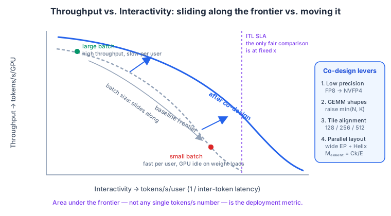
Two consequences follow:
- A single number is meaningless. “Tokens per second” without a stated ITL target is unfalsifiable. The honest comparison is frontier-vs-frontier, and the honest scalar summary is the area under the frontier — the envelope of achievable operating points.
- Co-design is frontier expansion, not point optimization. Quantization, wider-shallower aspect ratios, and better parallel decompositions all push the whole curve out and to the right, which is qualitatively different from sliding along it by changing batch size. This is the same framing as the roofline tour in The Economics of a Token and the vendor comparison in The State of Scaling LLM Inference.
Workload regimes and Amdahl’s Law
Where you sit on the frontier determines which part of the model to optimize. The 2×2 is context length (short vs. long) crossed with the objective (throughput vs. latency):
| Short context | Long context | |
|---|---|---|
| Throughput-first | FFN/MoE GEMMs dominate; weight traffic amortized by large $C$ | Attention $\mathcal{O}(S)$ per token plus KV-cache bandwidth begins to rival FFN |
| Latency-first | Weight-load bound; the whole model streams from HBM per step | KV-cache-read bound; attention is the critical path |
Amdahl’s Law is the discipline here. If attention consumes a fraction $f$ of step time and you accelerate everything else by $k$:
\[S(k) = \frac{1}{f + \frac{1-f}{k}}, \qquad \lim_{k\to\infty} S(k) = \frac{1}{f}.\]At $f = 0.4$ — a plausible long-context decode split — an infinitely fast FFN buys $2.5\times$. Optimizing the FFN in that regime is capped before you start; the leverage is in the attention and KV path, which is exactly the argument behind sparse-attention index reuse in IndexCache and the asymmetric-scaling analysis in FlashAttention-4.
2. Transformer Layers as GEMM Shapes
The primitive
Everything reduces to $C = AB$ with $A \in \mathbb{R}^{M \times K}$, $B \in \mathbb{R}^{K \times N}$, $C \in \mathbb{R}^{M \times N}$:
\[\text{FLOPs} = 2 \cdot M \cdot N \cdot K,\] \[\text{ReadBytes} = M K \cdot b_A + K N \cdot b_B, \qquad \text{WriteBytes} = M N \cdot b_C,\]with $b_X$ the bytes per element of operand $X$. The quantity that decides whether the GEMM is compute- or memory-bound is arithmetic intensity:
\[I = \frac{\text{FLOPs}}{\text{Bytes}} = \frac{2MNK}{b_A MK + b_B KN + b_C MN}.\]A kernel is compute-bound when $I$ exceeds the machine’s ridge point $I^\star = \text{peak FLOP/s} \,/\, \text{peak bytes/s}$.
Layer-by-layer shape map
Let $T$ be the number of tokens in the GEMM (batch × sequence for prefill, batch for decode), $H$ the hidden dimension, $H’$ the FFN/expert intermediate dimension, $n_q$ / $n_{kv}$ the query / KV head counts and $d_h$ the head dimension.
| Layer | $M$ | $N$ | $K$ |
|---|---|---|---|
| QKV projection | $T$ | $(n_q + 2 n_{kv}) d_h$ | $H$ |
| Attention output projection | $T$ | $H$ | $n_q d_h$ |
| FFN-1 (gate + up) | $T$ | $2H’$ | $H$ |
| FFN-2 (down) | $T$ | $H$ | $H’$ |
Two structural facts jump out. First, $M$ is always the token count — it is the only dimension the serving system controls at runtime; $N$ and $K$ are frozen by the architecture. Second, the down-projection is the odd one out: it is the only layer whose reduction dimension $K$ is the small intermediate $H’$ rather than the large hidden $H$.
The “square block” result
Consider the balanced case $M = N = K = H$ with a uniform $b$ bytes per element:
\[I = \frac{2H^3}{3bH^2} = \frac{2H}{3b}.\]Arithmetic intensity grows linearly in $H$. Doubling the hidden dimension doubles the FLOPs per byte moved — this is why large models are, counterintuitively, easier to run efficiently than small ones, and why the trend toward wide models is hardware-friendly rather than merely capacity-driven.
The intensity cap: why FFN-2 stays memory-bound
Now take the batching limit. As $M \to \infty$ the weight-load term $b_B KN$ becomes negligible and
\[I_\infty = \frac{2MNK}{b\,M K + b\,M N} = \frac{2}{b}\cdot\frac{NK}{N + K}.\]The right-hand factor is (half) the harmonic mean of $N$ and $K$, which is dominated by whichever is smaller. When $K \ll N$:
\[I_\infty \approx \frac{2K}{b}.\]No amount of batching escapes this. The ceiling is set by the smaller of the two architectural dimensions, not by the token count.
Case study — an MoE down-projection on GB300. Take an expert with $H’ = 512$, $H = 8192$, executed in NVFP4 so $b = 0.5$ bytes:
\[I_\infty = \frac{2}{0.5}\cdot\frac{8192 \cdot 512}{8192 + 512} = 4 \cdot \frac{4{,}194{,}304}{8704} \approx 1{,}930 \ \text{FLOP/byte}.\]A GB300-class GPU sits at roughly $15$ PFLOP/s dense FP4 against roughly $8$ TB/s of HBM3e, so
\[I^\star \approx \frac{15 \times 10^{15}}{8 \times 10^{12}} \approx 1{,}900 \ \text{FLOP/byte}.\]The layer lands at the ridge point in the idealized limit — and in practice below it, once you account for the epilogue writing FP32 or BF16 accumulators, scale-factor traffic, imperfect L2 reuse, and the fact that $M$ is finite. The conclusion is architectural, not a kernel bug: an expert intermediate of 512 cannot saturate a modern FP4 Tensor Core. Widening $H’$ to 2048 lifts the cap to roughly $6{,}500$ FLOP/byte, comfortably compute-bound, at the cost of a wider expert. This is the quantitative version of the pressure toward fewer-but-fatter experts, and it interacts directly with the megakernel fusion strategy in Mixture-of-Kittens — if the layer is bandwidth-bound anyway, fusing away intermediate round-trips is the only remaining lever.
Note also the precision coupling: $I_\infty \propto 1/b$. Going from BF16 to NVFP4 raises arithmetic intensity by $4\times$ while raising peak FLOP/s by roughly the same factor, so the ridge point moves too. Low precision does not automatically fix a memory-bound layer; it moves both sides of the inequality.
3. Microarchitecture Alignment: Tiles, Clusters, and Aspect Ratio
Tile-based execution
A GEMM is decomposed into output tiles of shape $(B_M, B_N)$, each assigned to a Streaming Multiprocessor — or, on Blackwell, to a cluster of SMs cooperating through clusterMMA and CGA-scoped shared memory, with distributed tile scheduling handled in hardware (Cluster Launch Control, Blackwell SM100).
Tile quantization
The efficiency loss from ragged edges is exact and easy to compute:
\[\eta_{\text{tile}} = \frac{M \cdot N}{B_M \left\lceil \tfrac{M}{B_M} \right\rceil \cdot B_N \left\lceil \tfrac{N}{B_N} \right\rceil}.\]With $B_N = 128$ and $N = 640$, $\eta = 1$. With $N = 641$, the kernel launches a sixth tile column for a single useful column: $\eta = 641/768 \approx 0.83$. A one-element change in a config file costs 17% of the machine.
Wave quantization is the same phenomenon one level up. With $P$ SMs (or clusters) and $\mathcal{T}$ tiles:
\[\eta_{\text{wave}} = \frac{\mathcal{T}}{P \left\lceil \mathcal{T}/P \right\rceil}.\]At $P = 148$ and $\mathcal{T} = 150$, two waves run to do the work of one plus two tiles: $\eta \approx 0.51$. Small GEMMs are especially exposed.
The alignment ladder. Dimensions should be multiples of:
- 128 — the base MMA tile floor;
- 256 — clusterMMA, where two SMs cooperate on one tile;
- 512 — a four-SM CGA.
The subtlety is that the relevant quantity is the dimension after parallel sharding. A hidden size of 8192 is beautifully aligned; sharded across TP=6 it becomes $1365.\overline{3}$ — not an integer, let alone a multiple of 128. Architectural dimensions must be divisible by $128 \times \text{TP}$ (or $\times \text{EP}$, $\times \text{SP}$) for every deployment configuration you intend to support. Choosing $H$, $H’$, $n_q$, $n_{kv}$ as products of small powers of two is not superstition; it is what keeps the deployment space non-empty.
Width versus depth
For a fixed parameter budget, the aspect ratio $H/L$ ($L$ = layer count) is nearly free from the loss’s point of view over a broad range — but the hardware is not indifferent:
- Critical path. Decode latency is $L$ serial layer executions, each with kernel-launch, synchronization, and (in tensor-parallel deployments) a collective. That per-layer fixed cost $\tau$ makes step time $\approx L(t_{\text{math}} + \tau)$. Halving $L$ halves the $\tau$ term outright.
- Weight reuse and tile occupancy. Wider layers mean larger $N$ and $K$, higher $I$ (Section 2), and fewer edge tiles.
- Communication. Tensor-parallel all-reduce volume per layer scales with $H$, but the count of collectives scales with $L$ — and at small message sizes latency, not bandwidth, dominates (NCCL GIN & MSCCL++).
Against this, depth buys representational power: sequential composition is not replaceable by width, as the length-generalization results in Looped Transformers make clear. The co-design recommendation is to sit at the wide end of the region where loss is flat in $H/L$ — take the free hardware win where the quality curve is indifferent, not beyond it.
4. Quantization: The Cheapest Frontier Expansion
The lever
Dense Tensor Core throughput roughly doubles at each precision step, FP16/BF16 $\to$ FP8 $\to$ NVFP4, and memory footprint and bandwidth demand fall proportionally. For a weight-bound decode step — the common case at low batch — halving the bytes per weight nearly halves the step time. No architectural change delivers that ratio as cheaply.
NVFP4 micro-block scaling
NVFP4 stores values as E2M1 (1 sign, 2 exponent, 1 mantissa bit) with a two-level scale hierarchy:
\[x_{i} \;\approx\; s_{\text{tensor}} \cdot s_{\text{block}(i)} \cdot q_i, \qquad q_i \in \text{E2M1},\]where $s_{\text{block}}$ is an FP8 (E4M3) scale shared by a 16-element micro-block and $s_{\text{tensor}}$ is a single FP32 per-tensor scale. Effective storage:
\[4 + \frac{8}{16} = 4.5 \ \text{bits/value}.\]The design trades a slightly larger scale budget than MXFP4 (32-element blocks with E8M0 power-of-two scales, $4.25$ bits/value) for two things that matter for accuracy: a finer block (16 vs. 32 values, so a single outlier corrupts half as many neighbors) and a non-power-of-two scale (E4M3 has mantissa bits, so the block scale can land near the true block maximum instead of rounding up to the next power of two, wasting up to a full exponent step of dynamic range). The per-tensor FP32 factor then re-centers the whole tensor into the E4M3 scale’s representable range.
Accuracy in practice
The empirical result that makes this deployable is that a strong reasoning model — DeepSeek-R1 is the reference case — retains accuracy close to its FP8 baseline across reasoning and knowledge benchmarks under NVFP4 post-training quantization, with the residual gap recoverable by quantization-aware methods. The methodology behind those recoveries is covered in Quantization-Aware Distillation for NVFP4 and the checkpoint-production side in Creating the Nemotron 3 Ultra NVFP4 Checkpoint; the training-time story is in NVFP4: Stable 4-Bit Training, and the RL-loop complications — where a quantized generator and a higher-precision trainer disagree — in The 4-bitter Lesson.
The co-design point: quantization is only “free” if the architecture cooperates. Micro-block scaling assumes the reduction dimension is a multiple of 16; per-tensor scaling assumes outliers are bounded, which is a statement about the activation function and normalization placement, not about the number format. Architectures that softcap their GLU branches are, among other things, easier to quantize.
5. Multi-GPU Parallelism: Getting $M$ Large Enough
Section 2 established that $M$ is the only shape dimension the runtime controls. Section 5 is about how the parallel decomposition determines what $M$ each GPU actually sees.
MoE and expert parallelism
Under uniform routing, a global batch of $C$ concurrent tokens with top-$k$ routing over $E$ experts gives each expert an expected GEMM $M$ of:
\[M_{\text{expert}} = \frac{C \cdot k}{E}.\]This is the central sizing equation of MoE serving. Suppose the tile and intensity analysis says you need $M^\star = 256$ tokens per expert for a compute-bound GEMM. Then:
\[C \;\ge\; \frac{M^\star \cdot E}{k}.\]With $E = 256$ and $k = 8$: $C \ge 8{,}192$ concurrent tokens. A sparse model with many experts is only efficient at very high concurrency — which is precisely the argument for wide expert parallelism spanning a whole NVL72 rack, and why MoE serving economics are so different from dense serving. The parallelism-folding trade-offs are worked out in MoE Parallel Folding, and the production form in DeepSeek-V4 on Blackwell.
Real routing is not uniform. If the busiest expert receives $(1+\delta)$ times the mean, the step is gated by that expert and effective utilization falls by roughly $1/(1+\delta)$ — which is why auxiliary-loss-free load balancing and quantile-style routing corrections are systems features, not regularization details.
Chunked pipeline parallelism
Pipelining across $S$ stages with $m$ chunks in flight leaves a bubble fraction
\[\text{bubble} = \frac{S-1}{S-1+m},\]provided the stages are balanced. They usually are not: with hybrid architectures mixing attention layers, linear-attention layers, and MoE layers, an even split by layer count is an uneven split by time. The fix is to assign layers to stages by measured cost so that per-stage latency — not per-stage depth — is equalized. Under prefill/decode disaggregation (Disaggregate Prefill and Decoding) this must hold in both regimes, whose cost profiles differ: prefill is FFN-heavy and compute-bound, decode is KV-heavy and bandwidth-bound. A stage partition tuned for one is wrong for the other, which is an argument for disaggregating the partition as well as the phase.
Hybrid schemes: decoupling attention from FFN
The classical bottleneck: tensor parallelism for attention cannot exceed the KV head count $n_{kv}$ without duplicating the KV cache across ranks. With GQA at $n_{kv} = 8$, TP=16 means every KV byte is stored twice — and the KV cache is exactly what long-context decode is bound on.
The resolution is to stop insisting that attention and FFN use the same decomposition:
- FFN/MoE shards over the intermediate dimension (TP) or over experts (EP), where the natural degree is large.
- Attention shards over the sequence dimension — Helix Parallelism — so each rank owns a contiguous slice of the KV cache regardless of $n_{kv}$. Each rank computes partial attention over its slice; the results combine with a log-sum-exp reduction, the same associative online-softmax merge that FlashAttention uses across tiles.
KV bytes per rank become
\[\frac{2 \cdot L \cdot n_{kv} \cdot d_h \cdot b_{kv} \cdot S}{P_{\text{seq}}},\]which scales with the shard count rather than being floored by $n_{kv}$. The cost is a layout change between the attention and FFN blocks — an all-to-all per layer, whose latency at small message sizes is a real tax and the reason low-latency collectives are part of the co-design story (Inside TPU and GPU Clusters, How to Think About GPUs). It is also why sequence-dimension sharding shows up independently in training (Scaling Video Training with SP).
Takeaways
- Optimize the frontier, not a point. Tokens/s/user and tokens/s/GPU trade against each other along a curve; co-design is what moves the curve, batch size only slides along it.
- Apply Amdahl before optimizing. In long-context decode, an infinitely fast FFN is worth $1/f$. Know $f$ first.
- Arithmetic intensity is capped by the smallest architectural dimension, $I_\infty \approx 2\min(N,K)/b$. A 512-wide expert intermediate cannot saturate an FP4 Tensor Core no matter how large the batch.
- Align to 128 / 256 / 512 — after sharding. Tile and wave quantization turn off-by-one dimensions into double-digit efficiency losses, and the constraint applies to $H/\text{TP}$, not $H$.
- Prefer the wide end of the flat region. Depth costs serial latency, per-layer collectives, and tile occupancy; take the width where loss is indifferent.
- NVFP4’s 4.5 bits/value buys $4\times$ throughput — but it raises the ridge point too, so it is not a cure for a structurally memory-bound layer.
- $M_{\text{expert}} = Ck/E$ is the MoE sizing equation. Many experts implies high required concurrency implies wide EP; load imbalance divides the result by $(1+\delta)$.
- Decouple the decompositions. Attention wants sequence sharding, FFN wants intermediate or expert sharding. Forcing one scheme on both is what makes KV cache duplication look inevitable.
The through-line is that hardware constraints are not downstream of architecture — they are a co-equal set of equations. The models that serve efficiently in 2027 will be the ones whose dimensions were chosen with the ridge point and the tile size on the whiteboard, in the same spirit as the hardware-aware design notes in DeepSeek-V3’s Hardware-Aware Design.