MAI-Base-2: Scaling Ladders, LR×WD Laws, and Co-Design for a 2.8T MoE
Reading notes on:
Microsoft AI’s pretraining update describes MAI-Base-2, a sparse MoE foundation model with 80B active and 2.8T total parameters, trained on 50T tokens on 16,000 GB200 GPUs in 38 days. The headline claim is efficiency: 4.2 to 12.3× more FLOPs-efficient than DeepSeek-V4-Pro-Base and 6.3 to 12.7× more than its predecessor MAI-Base-1 (the base model behind MAI-Thinking-1).
What makes the post worth reading is less the model than the method. It shows how to predict the final loss from a ladder of small runs to within 0.3%, a closed-form law for learning rate and weight decay, and the infrastructure that made an MoE in every layer and the Muon optimizer cheap enough to use at 16K GPUs.
1. Results at a Glance
Held-out loss (bits per byte, lower is better)
Test sets are held out and decontaminated against the training data.
| Domain | MAI-Base-2 | DeepSeek-V4-Pro-Base | Kimi-K3 | MAI-Base-1 |
|---|---|---|---|---|
| Code (MAI codebase) | 0.2203 | 0.2370 | 0.2264 | 0.2401 |
| QA | 0.4162 | 0.4351 | 0.4269 | 0.4440 |
| STEM | 0.3653 | 0.3968 | 0.3761 | 0.4026 |
| Math | 0.3561 | 0.3862 | 0.3589 | 0.3939 |
Kimi-K3 is the closest competitor on every domain (on math the gap is only 0.0028 BPB); see Kimi K3 for that model, which happens to have the same 2.8T total size. DeepSeek-V4-Pro-Base is the open-weight base the efficiency multiples are quoted against (DeepSeek-V4 architecture).
Training run
- 16,000 GB200 GPUs for 38 days (August to September 2026).
- 21% average MFU, measured against GB200’s 2.5 PFLOPS BF16 peak and excluding rematerialization and optimizer FLOPs, so it is a conservative number.
- 89% goodput.
These numbers are self-consistent. The usual $6ND$ estimate gives $6 \times 80\text{B} \times 50\text{T} = 2.4 \times 10^{25}$ FLOPs, while $16{,}000 \times 2.5\,\text{PFLOPS} \times 0.21 \times 38\,\text{days} \times 0.89 \approx 2.45 \times 10^{25}$. (For more on this kind of accounting, see Infra Math for LLM Training.)
2. Architecture: MAI-Base-1 vs MAI-Base-2
The big structural change is moving from alternating dense and MoE layers to an MoE in every layer, plus native vision.
| MAI-Base-1 | MAI-Base-2 | |
|---|---|---|
| Active / total params | 35B / 1T | 80B / 2.8T |
| Layers $L$ | 78 | 102 |
| Hidden dim | 6656 | 8704 |
| MoE layout | Alternating dense FFN and MoE | MoE in every layer |
| MoE down-projection dim | 3072 | 4096 |
| Expert FFN dim | 10240 | 8704 |
| Routing | 0 shared + 8 of 512 routed | 1 shared + 7 of 512 routed |
| Attention heads, global layers (every 6th), KV / Q | 8 / 80 | 2 / 96 |
| Attention heads, local layers, KV / Q | 8 / 80 | 16 / 96 |
| Embeddings | Tied | Untied |
| Tokens | 30T | 50T |
| Optimizer | AdamW | Muon (2D non-embedding params) + AdamW |
| FP8 | Tensor-wise delayed scaling, E4M3/E5M2 | MXFP8 E4M3 |
| Gradient clipping | Global weight-gradient | Global weight-gradient + activation-gradient |
| Modality | Text | Native VLM, encoder-free |
A few things stand out:
- Asymmetric KV heads. Global layers drop to just 2 KV heads while local layers go up to 16. The post doesn’t give the rationale, but it fits the cost structure: global layers are the ones whose KV cache grows with context, while local sliding-window layers have a bounded cache and can afford more heads. (Window layers are also where attention-sink behavior matters, see StreamingLLM.)
- A shared expert returns (1 shared + 7 routed instead of 8 routed), the same pattern as DeepSeek-V3 and successors.
- MXFP8 replaces tensor-wise delayed scaling: block-scaled E4M3 everywhere, without the scale-history bookkeeping. See MXFP8 Training.
- Muon for 2D matrices, AdamW for the rest, as in Kimi and DeepSeek-V4; SOAP, Muon, and Beyond covers the optimizer side.
3. Scaling Science
3.1 The scaling ladder
To forecast the big run without the small runs drifting architecturally, every rung of the ladder is defined by its layer count $L$, holding tokens per active parameter (TPP) constant:
\[d_{\text{model}} = \frac{256}{3} \cdot L, \qquad H_Q = \text{round}_{16}(L)\]Both production models sit exactly on this ladder: $L = 78$ gives $d = 6656$ and $H_Q = 80$ (MAI-Base-1), and $L = 102$ gives $d = 8704$ and $H_Q = 96$ (MAI-Base-2).
Source scaling. Small ladder runs see far fewer tokens, so naively they would see each data source fewer times than the real run, and they would never hit the multi-epoch effects the big run will. Source scaling shrinks the unique data so every sub-dataset is repeated exactly as many times as in the target run. For a 1/10-scale run, if the full run repeats a source 8 times, the small run repeats 1/10 of that source 8 times. This keeps the ratio of unique data to active parameters constant across rungs.
It worked. A log-log power law fit on rungs $L18$ through $L42$ predicted a final NLL of 0.8034. The real run finished at 0.8058, a +0.3% error. (Compare the methodology in Deconstructing Scaling Laws and The Architecture of Scaling Laws.)
3.2 Hyperparameter laws
Loss is mostly sensitive to the product of learning rate and weight decay, so a rectangular LR × WD grid wastes most of its points off the good diagonal band. Instead the sweep uses rotated coordinates:
\[\left( \log \text{LR},\; \log(\text{LR} \times \text{WD}) \right)\]A 2D quadratic fit to NLL across 15 experiment groups gives closed-form optima:
\[\text{LR}^* \times \text{WD}^* = \frac{17.04}{\text{steps}}\] \[\log \text{LR}^* = -1.51 + 0.175 \log \text{TPP} - 0.573 \log \text{steps}\] \[\text{Dropout} = \text{sigmoid}\left(0.526 \cdot (\log \text{ActiveParams} - 27.2)\right)\]Both exponents have a clean interpretation:
- The $1/\text{steps}$ law for LR × WD is what decoupled weight decay predicts. The decay timescale $\tau = 1 / (\text{LR} \times \text{WD})$ should be a fixed fraction of training, so the product must shrink in proportion to the number of steps.
- $\text{LR}^* \propto \text{steps}^{-0.573}$ is close to the classic square-root rule ($\text{steps}^{-0.5}$).
The dropout law is a sigmoid in log active parameters, so the optimal dropout rises smoothly with model size.
4. Infrastructure and Co-Design
Every recipe change is judged by its efficiency gain: how much less compute (or time) a candidate needs to reach the baseline’s eval loss.
\[\text{EG}_{\text{time}} = \frac{\text{Time}_{\text{baseline}}}{\text{Time}_{\text{candidate}}}, \qquad \text{EG}_{\text{FLOPs}} = \frac{\text{FLOPs}_{\text{baseline}}}{\text{FLOPs}_{\text{candidate}}}\]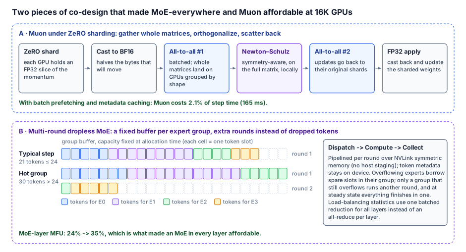
4.1 Multi-round dropless MoE
Putting an MoE in every layer only pays off if MoE layers run efficiently; MoE-layer MFU had to rise from 24% to 35%. The two standard approaches both lose: a fixed capacity threshold drops tokens when routing is imbalanced, and allocating for the worst case wastes memory.
MAI-Base-2 uses multi-round dropless MoE with fixed memory:
- Experts on each expert-parallel rank are grouped into expert groups with a configurable capacity.
- Work runs as a pipelined Dispatch → Compute → Collect schedule.
- An expert that overflows uses spare capacity from peers in its group; if the group still overflows, the leftover tokens run in additional deterministic rounds.
- At steady state, everything finishes in one round.
Overheads removed along the way:
- NVLink symmetric memory for direct GPU-to-GPU token transfer, with no host staging copies.
- Fewer kernel launches via grouped GEMMs and device-resident token metadata.
- Batched load balancing: one batched reduction across all layers instead of a load-balancing all-reduce per layer.
MAI-Base-1 had already gone dropless; this is the version that scales to MoE everywhere. For other takes on the same problem, see MoE in Megatron Core and UltraEP.
4.2 Muon at 16K GPUs
Muon orthogonalizes each weight matrix’s momentum with Newton–Schulz iterations, which need the whole matrix. ZeRO shards every matrix across GPUs. The resolution:
- Cast local FP32 momentum shards to BF16.
- A batched all-to-all sends each full matrix to one GPU, grouping matrices by shape.
- Each GPU runs symmetry-aware Newton–Schulz on its full matrices.
- A second all-to-all returns the updates to their ZeRO shards, which cast back to FP32 and apply them.
With batch prefetching and metadata caching, Muon costs 2.1% of step time (165 ms). veScale-FSDP tackles the same mismatch between matrix-shaped optimizers and flat parameter shards from the FSDP side.
4.3 Activation-gradient clipping
Global weight-gradient clipping is blunt: one outlier scales down the whole update. Activation-gradient clipping clips the gradients flowing through activations at selected interior layers, so an outlier is contained locally instead of shrinking the entire update.
- Stability: gradient norms stay in a tight band for the whole run (median 0.0233 to 0.0759, with no large spikes).
- Gets better with scale: +28% FLOPs efficiency gain at $L42$.
- A data-bug detector: clipping events helped find a preprocessing bug that truncated code pull requests mid-sentence at a Gradle license header.
5. Data
50T training tokens (36% more unique text tokens than MAI-Base-1), knowledge cutoff March 2026, all organic, with no distillation from external models.
| Source | Share of tokens | Growth in unique tokens vs MAI-Base-1 |
|---|---|---|
| Code | 45% | +34% |
| Vision (encoder-free VLM) | 18% | 4.5T unique tokens (new modality) |
| Web | 12% | +16% |
| PDFs and documents | 9% | +104% |
| STEM | 9% | +24% |
| Books | 5% | +194% |
| Math | 4% | +37% |
| Other | 2% | +22% |
The shares as listed add up to 104%, so treat them as approximate. Even so, the direction is clear: code is by far the largest slice, and the fastest-growing sources are long-form (books nearly tripled, PDFs doubled).
6. Principles
- Learn from organic data. Capability should come from high-provenance pretraining data, not distillation from other models.
- Prefer methods that transfer. Source scaling and activation clipping were chosen because their gains carry predictably from ladder rungs to the full run.
- Co-design model and infrastructure. MoE everywhere was only adopted once multi-round dropless MoE made it efficient, and Muon only once it fit ZeRO for 2.1% overhead.
Takeaways
- Ladders that don’t drift predict well. Tying width and heads to depth ($d = 256L/3$, $H_Q = \text{round}_{16}(L)$), fixing TPP, and source-scaling the data gave a 0.3% final-loss prediction error.
- Sweep LR and WD along their product. $\text{LR}^* \times \text{WD}^* = 17.04/\text{steps}$ is decoupled weight decay’s constant-timescale rule, measured.
- MoE in every layer is an infrastructure decision. It required raising MoE-layer MFU from 24% to 35% without dropping tokens.
- Muon scales if you move whole matrices. Two all-to-alls around ZeRO shards cost 2.1% of step time at 16K GPUs.
- Clip activation gradients, not just weight gradients. It stabilizes training, helps more at larger scale (+28% at $L42$), and surfaces data bugs.