MergeKit: Model Merging as a Memory-Bound Systems Problem
Reading notes on:
Model merging is one of the few techniques in the post-training toolbox with no training loop in it at all. You take two or more checkpoints, you do arithmetic on their parameter tensors, and you get a third checkpoint. No gradients, no data, no optimizer state, no cluster.
That framing makes the algorithm sound like the interesting part, and it is where most of the literature lives. MergeKit’s contribution is to point out that once you actually want to do this at 70B, the algorithm is nearly free and the memory schedule is the whole problem. Merging two 70B models naively means holding 280 GB of bf16 weights resident to produce a 140 GB output. The toolkit’s answer is to compile the merge recipe into a DAG and stream tensors through it, which turns a cluster job into something you can run on a workstation.
So there are two things worth reading here: a taxonomy of what merging methods actually do to parameters, and an execution architecture for running them out-of-core.
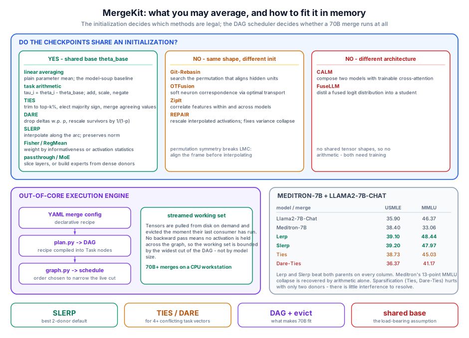
1. The Taxonomy: What Are You Allowed to Average?
The organizing question is not “which method is best” but what relationship do the input checkpoints have to each other. MergeKit splits the space along two axes, weight initialization and architecture, and the first axis is the one that decides whether parameter-space arithmetic is legal at all.
1.1 Identical architecture, shared initialization
This is the easy regime, and it is the one nearly all practical merges live in: several checkpoints all fine-tuned from one base model. The justification is Linear Mode Connectivity (LMC): checkpoints descended from a shared base stay inside one loss basin, connected by low-loss linear paths, so the segment between them is not garbage.
That is the same property that makes weight averaging work in Averaging the Sweep, and merging is best understood as the generalization of soups from “one task, many hyperparameters” to “many tasks, one base”.
Linear weight averaging / model soups. Average the parameters directly. The baseline every other method is trying to beat.
Task arithmetic. Define the task vector
\[\tau_i = \theta_i - \theta_{\text{base}}\]as the parameter displacement a fine-tune induced relative to the shared base. Task vectors turn out to be composable objects: you can add them to stack capabilities, scale them to modulate strength, and negate them to subtract a behavior. The merged model is $\theta_{\text{base}} + \sum_i \lambda_i \tau_i$.
TIES (Trim, Elect Sign, Merge). Adding task vectors naively suffers interference: two fine-tunes that both want to move a parameter, in opposite directions, cancel each other into mush. TIES attacks this in three steps:
- Trim: sparsify each $\tau_i$ to its top-$k\%$ highest-magnitude entries, on the theory that small entries are noise.
- Elect sign: per parameter, take the majority sign across the surviving task vectors.
- Merge: average only the values that agree with the elected sign, discarding the dissenters.
The insight is that sign conflict, not magnitude, is what destroys merges.
DARE (Drop And REscale). A cheaper sparsification: drop entries of $\tau_i$ independently with probability $p$, and rescale the survivors by $\frac{1}{1-p}$ so the expected task vector is unchanged. It is dropout applied to the delta rather than to activations, and the rescale is what keeps it unbiased. DARE composes with TIES (the dare_ties method), which is where most practical recipes end up.
SLERP (spherical linear interpolation). Linear interpolation between two parameter vectors shrinks the norm of the result whenever the vectors are not collinear: the midpoint of two unit vectors at $90°$ has norm $\frac{1}{\sqrt 2}$, not 1. SLERP interpolates along the arc instead, preserving norm and treating the interpolation as a rotation rather than an average. For two-model merges this is usually the strongest default, and the case study below bears that out.
Data-informed weighting. Rather than weighting every parameter equally, weight by how much it matters:
- Fisher merging weights parameters by Fisher information, i.e. by how sharply the loss responds to perturbing them.
- RegMean solves for merge weights in closed form by minimizing L2 distance between the merged model’s layer outputs and the originals, using only local input activation statistics, so it needs activations but not raw training data.
Structural merges. These do not combine parameter values at all:
- Passthrough / layer slicing (“FrankenMerging”) concatenates layer ranges from different models into a deeper stack. Goliath-120B and the depth up-scaling behind SOLAR-10.7B are built this way.
- Franken-MoE (
mergekit-moe) assembles a sparse MoE from several dense models, one expert per donor, with router gates initialized either randomly (sparse up-cycling) or from semantic hidden-state heuristics over prompt exemplars. It is a way to get an MoE without the routing machinery being trained end to end.
Evolutionary merging. Merge recipes have many free knobs and no gradient, so search them. Evolutionary methods optimize jointly over parameter space (which weights, which coefficients) and data flow space (which layers, in what order), which is how you discover a passthrough+arithmetic hybrid nobody would write by hand.
1.2 Identical architecture, different initializations
Here LMC fails, and it fails for a structural reason: neural networks have permutation symmetry. Reorder the hidden units of a layer (and correspondingly the rows/columns of the adjacent weight matrices) and you get a functionally identical network with completely different parameter tensors. Two independently initialized models are almost surely in different permutation frames, so averaging them aligns unit 7 of one with unit 7 of the other for no reason at all.
The methods in this bucket all try to fix the frame before interpolating:
- Git-Rebasin / neuron alignment searches for the permutation that best aligns one model’s units to the other’s, then interpolates.
- OTFusion relaxes hard permutation to a soft correspondence via optimal transport.
- ZipIt merges by correlating features both across models and within a single model, which lets it fuse networks trained on genuinely different tasks.
- REPAIR patches a second-order symptom: interpolated layers have collapsed activation variance relative to their endpoints, so rescale the statistics back.
This bucket is well-studied and rarely used in LLM practice, because in practice you always do have a shared base.
1.3 Different architectures
Once the parameter shapes do not match, there is nothing to average. CALM composes two models with trainable cross-attention between them; FuseLLM distills a fused output distribution from several teachers into a student. Both work, and both require a training phase, which forfeits the entire premise of merging. They belong in the same family as the behavioral-transfer approach in Breaking the Tokenizer Barrier: when parameter arithmetic is unavailable, you fall back to matching behavior.
2. The Execution Engine
The systems half. A merge is a pure function of tensors, which means the naive implementation (load everything, compute, save) is also the maximally memory-hungry one. MergeKit’s architecture is built around never doing that.
YAML → plan → DAG → schedule. A declarative merge config is compiled by the planner into a directed acyclic graph of Task nodes. Each task is a small tensor operation with declared dependencies. Because the graph is explicit and acyclic, the scheduler can choose an execution order that minimizes the number of simultaneously live tensors, rather than inheriting whatever order the config happened to be written in.
Out-of-core execution. Tensors are streamed lazily from disk on demand, and (the part that actually matters) evicted the instant their last downstream consumer has run. A merge of two 70B models never needs more than a few layers’ worth of tensors resident. This is what puts 70B+ merges on consumer hardware, including CPU-only boxes with ordinary RAM.
The interesting property is that per-tensor merging is embarrassingly streamable in a way training never is: there is no backward pass, so no activation has to be kept alive across the graph. The working set is bounded by the widest cut of the DAG, and the scheduler’s job is to keep that cut narrow.
Extension points. The codebase is organized so that each of those responsibilities is one file:
| Module | Responsibility |
|---|---|
merge_methods/base.py |
Interface for a new parameter transformation |
plan.py |
Declarative config → computational DAG |
graph.py |
Execution graph, scheduling, eviction |
architecture.py |
Normalizes heterogeneous HF architecture maps into one tensor-naming scheme |
architecture.py deserves the callout. The reason a merge tool is not a fifty-line script is that “the same” tensor is named differently across checkpoint families, and a merge across two families needs that normalized before any arithmetic happens.
3. Case Study: Meditron + Llama2-Chat
The empirical section merges Meditron-7B, a medical-domain continued-pretrain of Llama-2-7B, back into Llama2-7B-Chat, using four methods, and evaluates on three medical and three general benchmarks.
| Model / merge | USMLE | MedMCQA | PubMedQA | ARC-C | HellaSwag | MMLU |
|---|---|---|---|---|---|---|
| Llama2-7B-Chat | 35.90 | 35.45 | 73.40 | 44.20 | 55.40 | 46.37 |
| Meditron-7B | 38.40 | 24.07 | 71.40 | 40.20 | 54.50 | 33.06 |
| MeditronLlama-7B-Lerp | 39.10 | 36.65 | 75.60 | 46.76 | 58.66 | 48.44 |
| MeditronLlama-7B-Slerp | 39.20 | 36.91 | 75.60 | 46.84 | 58.67 | 47.97 |
| MeditronLlama-7B-Ties | 38.73 | 32.27 | 75.60 | 45.05 | 58.23 | 45.03 |
| MeditronLlama-7B-Dare-Ties | 36.37 | 27.56 | 72.20 | 42.92 | 54.79 | 41.17 |
Three things fall out of this table.
The merge beats both parents, everywhere. Not “trades off between them”; beats them. On USMLE the merges reach 39.20 against 38.40 for the medical specialist and 35.90 for the chat model. On MMLU they reach 48.44 against 46.37 for chat and 33.06 for the specialist. There is no column where the best merge loses to the better parent. That is the strongest claim in the paper and it is worth being slightly suspicious of; the natural reading is that Meditron’s domain pretraining learned real medical knowledge while catastrophically forgetting instruction-following, and the merge recovers the latter without paying back the former.
Catastrophic forgetting is recoverable by arithmetic. Look at Meditron-7B’s MMLU: 33.06, a 13-point collapse from the chat model’s 46.37, on a benchmark that has nothing to do with medicine. That is the cost of narrow continued pretraining. Merging puts it back, and then some, without retraining. If you run a domain-adaptation pipeline, this says the last step should be merging the adapted weights back toward the generalist, not shipping the adapted weights.
SLERP wins, DARE-TIES loses, and the ordering is informative. SLERP edges Lerp on five of six columns; TIES trails both; DARE-TIES trails everything and on MedMCQA (27.56) and MMLU (41.17) is barely better than the specialist parent. The pattern is that sparsification hurts when you only have two models to merge. TIES and DARE exist to resolve interference between many task vectors; with two donors there is little interference to resolve, so trimming and dropping just throws away signal. Use TIES/DARE when merging four or five task-specific fine-tunes; use SLERP for a two-way blend.
4. A Scope Note on the Math
Worth stating plainly, because it shapes how you should read the taxonomy above: the MergeKit manuscript gives conceptual and architectural descriptions of TIES sign election, DARE Bernoulli masking, and SLERP geometry, and cites the originating papers for each rather than re-deriving them. The task-vector definition $\tau_i = \theta_i - \theta_{\text{base}}$ and the DARE rescale $\frac{1}{1-p}$ are the only algebra the paper itself commits to. If you want the full derivations (the TIES interference analysis, the DARE unbiasedness proof, the SLERP arc formula), they live in the original works, not here.
This is a toolkit paper. The novelty is the DAG and the out-of-core engine; the methods are a well-organized survey.
5. Takeaways
The interesting engineering is the scheduler, not the arithmetic. Every merge method in the taxonomy is a handful of elementwise tensor ops. What separates “works in a notebook on 7B” from “works on 70B on a workstation” is the DAG-plus-eviction discipline, and that is a general lesson: for any pure-function-of-weights transformation (merging, quantization, pruning, format conversion), the memory schedule is the product.
Pick the method by donor count, not by recency. Two donors from a shared base: SLERP. Four or more task vectors with real conflict: TIES, optionally with DARE on top. Different initializations: you need permutation alignment first and you should expect it to be fiddly. Different architectures: you are training something, so budget for it.
Merging is the cheap fix for domain-adaptation forgetting. The Meditron result is the practically useful one. A continued-pretrain that gains 2.5 points on USMLE and loses 13 on MMLU is not obviously a good trade, until you notice you can merge the general capability back in for the cost of one pass over the weights.
The scope condition is the same one soups have. Everything in §1.1 rests on a shared $\theta_{\text{base}}$ and the basin it defines. That is the load-bearing assumption, and §1.2 is the whole subfield that exists because it stops being true.