TailSFT: Stop Fitting What You Already Fit, and RL Gets a Better Start
Reading notes on:
The standard post-training pipeline runs pretraining → SFT → RL, and each stage is tuned on its own terms. SFT is judged by cross-entropy and pass@1. RL is judged by final reward. The trouble is that fitting SFT cross-entropy well can make the model a worse starting point for RL.
Cross-entropy keeps rewarding the model for raising the likelihood of demonstrations it can already generate easily. That sharpens the distribution toward the easy, well-modeled solutions and drains probability from valid alternatives the base model could also produce. RLVR then samples a group of rollouts per prompt. If every rollout fails, the group advantage is zero and the prompt produces no gradient at all. RL can only reinforce what the initialization can sample within its rollout budget, so an SFT checkpoint that has lost coverage has lost learning signal before RL even starts.
This is the same failure that When High SFT Scores Mislead diagnosed across hundreds of models: pass@1 measures the mode, and RLVR consumes the support. That paper tells you which checkpoint to hand over. TailSFT changes how the checkpoint is trained. SFT stops updating on sequences whose loss has already dropped a lot relative to the base model, and spends its gradient on the under-fit tail.
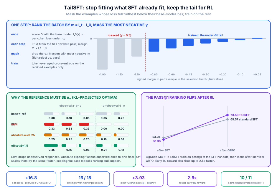
On OLMo-3 7B the trade is explicit. TailSFT accepts higher cross-entropy and sometimes lower pass@1, and in return raises pre-RL pass@16 by up to +16.8 points. After GRPO that becomes up to +3.9 points of pass@1, with early RL reward rising up to 2.5× faster.
1. Coverage, Formally
The coverage profile
For a target policy $\pi_D$, a model $\pi$, and prompts $x \sim \mu$, the coverage profile at scale $N$ is
\[\text{Cov}_N(\pi_D \parallel \pi) := \mathbb{P}_{x \sim \mu,\, y \sim \pi_D(\cdot \mid x)} \left[ \frac{\pi_D(y \mid x)}{\pi(y \mid x)} \ge N \right]\]This is the share of $\pi_D$’s mass that $\pi$ underweights by a factor of $N$ or more, so smaller is better. It maps directly onto a sampling budget. Prior work (Chen et al.) shows that if $\text{Cov}_N \le \tfrac{1}{2}$, then $K \ge 2N \log(1/\epsilon)$ samples are enough for Best-of-$K$ to get within $\text{Cov}_N + \epsilon$ of $\pi_D$’s expected reward.
pass@K as the measurable proxy
$\pi_D(y \mid x)$ is intractable, so in practice coverage is measured by pass@K at a $K$ comparable to the RL rollout budget:
\[\text{pass}@K(\pi) := \mathbb{E}_{x \sim \mu} \left[ 1 - (1 - p_\pi(x))^K \right], \qquad p_\pi(x) = \mathbb{P}_{y \sim \pi(\cdot \mid x)}[R(x, y) = 1]\]A model with lower cross-entropy and higher pass@1 can have worse large-$K$ pass@K. Those are the models that look best at the SFT handoff and start RL with the least signal.
2. The Algorithm: Offset Filtering Against $\pi_0$
TailSFT adds one comparison to standard SFT. It scores each example’s current loss against that example’s loss under the base policy $\pi_0$:
Algorithm 1: TailSFT (sequence-level relative filtering)
Require: base policy π₀, SFT dataset D, filtering schedule {γ_t}
1: Precompute base losses  ℓ₀(x_i) = -(1/|y_i|) log π₀(y_i | x_i)   for all (x_i, y_i) in D
2: for each training step t:
3:    Sample a selection batch B_t of size W·b   (W ranks, microbatch size b)
4:    Current losses          ℓ_t(x_i) = -(1/|y_i|) log π_t(y_i | x_i)
5:    Signed margin           m_t(x_i) = ℓ_t(x_i) - ℓ₀(x_i)
6:    F_t = the γ_t fraction of B_t with the most negative m_t   (fit the most, relative to base)
7:    Gradient step on B_t \ F_t with token-averaged cross-entropy:
         L_t(π) = Σ_{i ∈ B_t\F_t} -log π(y_i | x_i)  /  Σ_{i ∈ B_t\F_t} |y_i|
Three design choices matter:
- Length-normalized margins. Filtering uses per-token average loss, so selection is not biased toward long or short sequences.
- Relative, not absolute. An example is masked because its loss has fallen further below its own base loss than its peers’ have. Being low in absolute terms is not enough. An example the base model already found easy is not penalized for being easy. Only examples SFT has pushed hard get masked.
- Schedules. The filtered fraction is either a fixed $f$ or a linear ramp from 0 to $f$. The ramp guarantees every example is trained on early, before filtering starts to bite.
The cost is one scoring pass over the dataset with $\pi_0$ to store $\ell_0$. The current losses $\ell_t$ come from the forward pass SFT already runs. No reward model, no mode labels, no new objective. It is a mask applied to ordinary SFT.
3. Why the Reference Must Be $\pi_0$
The theory explains why filtering against $\pi_0$ beats filtering at an absolute loss threshold.
Setup: expert conditioning
Let $\pi_{\text{ref}}$ be the base distribution over responses and $S$ the set of rewarding responses. The expert conditions the base model on success:
\[\pi^\star(y) \propto \pi_{\text{ref}}(y) \cdot \mathbb{1}\{y \in S\}\]The dataset $\mathcal{D} = \{y_1, \dots, y_n\} \sim \pi^\star$ reveals an observed subset $\hat{S} \subseteq S$. Compare three objectives:
- ERM: $\mathcal{L}_{\text{ERM}}(\pi) = \frac{1}{n} \sum_i -\log \pi(y_i)$
- Absolute clipping: $\mathcal{L}_{\text{ABS},\alpha}(\pi) = \frac{1}{n} \sum_i \max\big(-\log \pi(y_i) + \log \alpha,\ 0\big)$, which stops pushing once $\pi(y_i) \ge \alpha$.
- Offset clipping (TailSFT): $\mathcal{L}_{\text{OFF},\beta}(\pi) = \frac{1}{n} \sum_i \max\big(-\log \pi(y_i) + \log(\beta\, \pi_{\text{ref}}(y_i)),\ 0\big)$, which stops pushing once $\pi(y_i) \ge \beta\, \pi_{\text{ref}}(y_i)$.
Each objective has many minimizers. The analysis picks the one closest to the base model:
\[\hat{\pi} = \arg\min_{\pi \in \Delta(\mathcal{Y})} \text{KL}(\pi \parallel \pi_{\text{ref}}) \quad \text{s.t.} \quad \mathcal{L}(\pi) = \min_{\pi'} \mathcal{L}(\pi')\]The KL projection is water-filling
Minimizing $\text{KL}(\pi \parallel \pi_{\text{ref}})$ subject to lower bounds $\pi(y) \ge f_y$ has Lagrangian
\[\sum_{y} \pi(y) \log \frac{\pi(y)}{\pi_{\text{ref}}(y)} + \lambda \Big(\sum_y \pi(y) - 1\Big) + \sum_y \mu_y \big(f_y - \pi(y)\big)\]Setting the derivative to zero gives $\pi(y) = \pi_{\text{ref}}(y)\, e^{-1-\lambda+\mu_y}$. By complementary slackness, unconstrained responses sit at a common scale $c\,\pi_{\text{ref}}(y)$ with $c = e^{-1-\lambda}$, and constrained ones sit exactly at $f_y$:
\[\hat{\pi}(y) = \max\big(f_y,\ c\, \pi_{\text{ref}}(y)\big), \qquad c \le 1 \text{ chosen to normalize}\]Plugging in each objective’s lower bound shows the difference:
-
Offset ($f_y = \beta\, \pi_{\text{ref}}(y)$ on $\hat{S}$):
\[\hat{\pi}_{\text{OFF},\beta}(y) = \begin{cases} \max(\beta, c)\, \pi_{\text{ref}}(y) & y \in \hat{S} \\ c\, \pi_{\text{ref}}(y) & y \notin \hat{S} \end{cases}\]Observed responses are scaled up uniformly, which keeps the base model’s relative preferences among them, and unobserved responses keep support.
-
Absolute ($f_y = \alpha$ on $\hat{S}$):
\[\hat{\pi}_{\text{ABS},\alpha}(y) = \begin{cases} \max\big(\alpha,\ c\, \pi_{\text{ref}}(y)\big) & y \in \hat{S} \\ c\, \pi_{\text{ref}}(y) & y \notin \hat{S} \end{cases}\]Every observed response is pushed to the same floor $\alpha$ regardless of how likely the base model found it, which overrides the base model’s own preferences.
The guarantee
For any $\pi_{\text{ref}}$, $S$, and sample:
\[\inf_{\beta}\, \text{Cov}_N(\pi^\star \parallel \hat{\pi}_{\text{OFF},\beta}) \;\le\; \min\Big\{ \text{Cov}_N(\pi^\star \parallel \hat{\pi}_{\text{ERM}}),\ \inf_{\alpha} \text{Cov}_N(\pi^\star \parallel \hat{\pi}_{\text{ABS},\alpha}) \Big\}\]Offset clipping is never worse than either alternative. The inequality can be strict, and absolute clipping can be strictly worse than plain ERM. So “stop training on examples with low loss” is not the idea. “Stop training on examples SFT has already moved far from the base model” is.
4. A Synthetic Warm-Up: Graph Navigation
A 10-layer DAG path-following task isolates the mechanism. The SFT data has a majority shard (7/8 of the mass) and a minority shard (1/8), each demonstrating a different rewarded path.
- Standard SFT anchors on the majority shard. It reaches the lowest cross-entropy (~0.60) and the highest pass@1 (~0.61), but pass@K stalls as $K$ grows, reaching pass@8 ≈ 0.97.
- Every filtering variant (absolute, quantile, and TailSFT) stops updating paths it has already fit, so it doesn’t over-concentrate. All of them reach pass@8 > 0.995, giving up single-sample accuracy for multi-sample coverage.
On this toy task all the filters look alike. The offset-vs-absolute distinction from Section 3 shows up on real language models, where base likelihoods vary by orders of magnitude across examples.
5. OLMo-3 7B: Coverage Before RL
TailSFT is evaluated on 18 dataset–benchmark pairs covering math (OpenMathInstruct-2, “OMI”) and code (BigCode, Magicoder, OpenCodeInstruct), with OLMES sampling. Selected rows:
| Domain | Dataset | Benchmark | SFT pass@1 | TailSFT pass@1 | SFT pass@16 | TailSFT pass@16 | Δ pass@16 |
|---|---|---|---|---|---|---|---|
| Math | OMI | AIME 2022–2025 | 3.65% | 4.03% | 15.24% | 18.31% | +3.07 |
| Math | OMI | MATH-500 Level 5 | 24.80% | 25.16% | 66.42% | 69.15% | +2.74 |
| Code | BigCode | MBPP+ | 53.04% | 51.36% | 74.69% | 78.84% | +4.14 |
| Code | BigCode | CruxEval-O | 4.16% | 13.18% | 24.21% | 41.00% | +16.79 |
| Code | Magicoder | CruxEval-I | 28.50% | 26.48% | 59.75% | 68.08% | +8.33 |
| Code | Magicoder | CruxEval-O | 12.86% | 16.16% | 38.08% | 47.92% | +9.83 |
TailSFT improves pass@16 in 15 of 18 settings. pass@1 moves both ways: it drops on BigCode MBPP+ and Magicoder CruxEval-I, where TailSFT de-prioritized examples the model already fit. The large-$K$ gains, by contrast, are consistent. By the SFT-stage leaderboard, several TailSFT checkpoints would lose.
6. After GRPO: The Coverage Pays Off
Matched standard-SFT and TailSFT initializations are each trained with GRPO under identical hyperparameters. Math uses the MATH train split (excluding MATH-500) with boxed-answer rewards. Code uses the MBPP+ train split with unit-test rewards.
| Benchmark | Init | Post-RL pass@1 | Post-RL pass@16 | Δ pass@1 |
|---|---|---|---|---|
| MATH-500 Level 5 | SFT | 57.70% | 83.83% | |
| TailSFT | 60.26% | 87.06% | +2.56 | |
| AIME 2022–2025 | SFT | 14.40% | 32.76% | |
| TailSFT | 15.61% | 36.06% | +1.21 | |
| BigCode MBPP+ | SFT | 69.57% | 75.93% | |
| TailSFT | 73.50% | 78.66% | +3.93 | |
| Magicoder MBPP+ | SFT | 70.52% | 78.22% | |
| TailSFT | 73.24% | 80.60% | +2.72 |
Two results stand out:
- The pass@1 ranking flips. On BigCode MBPP+, TailSFT trailed before RL (51.36% vs. 53.04% pass@1) and leads after it (73.50% vs. 69.57%). This is exactly the kind of checkpoint a pass@1-driven SFT handoff would throw away.
- RL starts faster. Training reward rises up to 2.5× faster from TailSFT initializations, because early rollout groups already contain successes and so produce non-zero advantages from the first steps.
Post-RL pass@16 also stays higher everywhere, so GRPO does not simply sharpen away the extra coverage. That fits the picture in Never Give Up: prompts with no successful rollouts give zero advantage and are never learned. NGU attacks this from the RL side by spending more samples on hard prompts. TailSFT attacks it from the SFT side by making sure those prompts are still sampleable when RL begins. The two are complementary.
7. A Diagnostic Before You Change Anything: $\rho_{16}$
Is standard SFT actually destroying coverage on your data? The coverage ratio answers that with nothing more than pass@1 estimates for $\pi_0$ and $\pi_{\text{SFT}}$.
Restrict to the base-reachable problems, $\mathcal{R}_0 = \{i : 0.05 < P_{i,16}(\pi_0) < 0.95\}$, which drops problems that are already saturated or out of reach. Map pass@1 to estimated pass@16 with $f_{16}(p) = 1 - (1-p)^{16}$, then add up the coverage standard SFT lost and gained:
\[L := \sum_{i \in \mathcal{R}_0} \Big[ f_{16}\big(P_{i,1}(\pi_0)\big) - f_{16}\big(P_{i,1}(\pi_{\text{SFT}})\big) \Big]^+, \qquad G := \sum_{i \in \mathcal{R}_0} \Big[ f_{16}\big(P_{i,1}(\pi_{\text{SFT}})\big) - f_{16}\big(P_{i,1}(\pi_0)\big) \Big]^+\] \[\rho_{16} := \frac{L}{G}\]- $\rho_{16} > 1$: SFT loses more base coverage than it gains, so TailSFT is likely to help. In 10 of 11 such settings TailSFT improved coverage (up to +28.7 points on a CruxEval-O setting), and the eleventh was unchanged.
- $\rho_{16} \le 1$: SFT is net-positive on base coverage. TailSFT may still help, or may be neutral.
It costs one standard SFT run plus pass@1 evaluation, which you probably already have.
Takeaways
- Cross-entropy keeps pushing on the head of the distribution. Once an example is fit, further CE pressure mainly sharpens the distribution and pulls mass from valid alternatives, and those alternatives are what RL needs to sample.
- Filter relative to the base model, not at an absolute loss. Offset clipping keeps $\pi_{\text{ref}}$’s relative preferences and provably covers at least as well as ERM or absolute clipping. Absolute clipping can be worse than doing nothing.
- Judge SFT checkpoints by large-$K$ pass@K. TailSFT’s pre-RL pass@1 is mixed, but its pass@16 wins 15 of 18 settings and turns into up to +3.9 points of post-GRPO pass@1 with up to 2.5× faster early RL, echoing the handoff metrics in When High SFT Scores Mislead.
- Check $\rho_{16}$ first. If standard SFT loses more coverage than it gains ($\rho_{16} > 1$), expect TailSFT to help.
- Optimize each stage for the next one. An intermediate checkpoint should be judged by how well it sets up the next stage, not by how well it scores on its own stage’s metric. Here that means SFT should leave the support intact for RL. It is the same reshaping-the-distribution view as in SFT, RL, and OPD through a distributional lens, applied to the handoff.