Set Block Decoding: Teaching One LLM to Predict Next Tokens and Fill In Masked Blocks
Reading notes on:
Autoregressive decoding is memory-bound. To produce one token, the GPU streams every weight and the whole KV cache out of HBM, then does very little arithmetic with them. That is why decoding a block of tokens in one forward pass costs almost the same as decoding one, and why so much inference research tries to emit more than one token per pass.
The usual routes each give something up. Speculative decoding and its relatives (Medusa, EAGLE) need a draft model or extra heads, and verification can only accept a contiguous left-to-right prefix. Masked diffusion LLMs decode many tokens in parallel but break exact KV caching and tend to lose quality.
Set Block Decoding (SBD) takes a third path. It fine-tunes an ordinary causal LLM so the same network does two jobs: standard next-token prediction (NTP) over the past, and masked token prediction (MATP) over a block of future positions, where any subset of the block may already be filled in. No architecture change, no extra heads, no draft model. Past tokens keep causal attention and an exact KV cache; only the block being decoded attends bidirectionally. On Llama-3.1 8B and Qwen-3 8B, SBD cuts forward passes by 3 to 5× with accuracy close to the NTP baseline.
1. From Next-Token Prediction to Set Parallel Decoding
An NTP model computes $p(x_t \mid x_{<t})$, one token per forward pass.
To decode a block $I = \lbrace t, \dots, t+k-1 \rbrace$ in one pass, you would want the joint $p(x_I \mid x_{<t})$, which has $\lvert V\rvert^k$ outcomes and is intractable. Multi-token approaches therefore approximate it with independent marginals,
\[p(x_I \mid x_{<t}) \approx \prod_{i \in I} p(x_i \mid x_{<t})\]That approximation is coarse, which is why speculative methods need an NTP verification pass that can only keep a contiguous prefix $x_t, \dots, x_{t+a}$.
Set parallel decoding relaxes the independence assumption step by step. Given any already-revealed subset $J \subset I$, predict each still-masked position $i \in M = I \setminus J$ from both the past and the revealed tokens:
\[p(x_i \mid x_{<t}, x_J), \qquad i \in M\]For any nested sequence of revealed sets $I_1 \subset I_2 \subset \dots \subset I_\ell = I$, decoding the new positions $D_j = I_j \setminus I_{j-1}$ in parallel at each step factorizes the block as
\[p(x_I \mid x_{<t}) = \prod_{j=1}^{\ell} \prod_{i \in D_j} p(x_i \mid x_{<t}, x_{I_{j-1}})\]This is exact whenever the tokens decoded together in one step are conditionally independent given everything revealed so far:
\[p(x_{D_j} \mid x_{<t}, x_{I_{j-1}}) = \prod_{i \in D_j} p(x_i \mid x_{<t}, x_{I_{j-1}})\]So the game is to reveal, at each step, a set of positions that are nearly independent, and the tokens need not be consecutive or in left-to-right order.
2. One Network, Two Modes
The SBD model $f_\theta(\cdot\,;\,\cdot)$ takes a causal part and an optional block part:
\[z_t = f_\theta(x_1, \dots, x_{t-1}\,;\,) \qquad \text{(autoregressive logits)}\] \[(\hat z_t, \dots, \hat z_{t+k-1}) = f_\theta(x_1, \dots, x_{t-1}\,;\, \hat x_t, \dots, \hat x_{t+k-1}) \qquad \text{(block logits)}\]Tokens left of the semicolon use causal attention and live in an ordinary KV cache. Tokens right of it attend bidirectionally within the block, and each $\hat x_i$ is either a real token or the mask token $m$. That gives two distributions from the same weights:
- NTP: $p_\theta(x_t \mid x_{<t}\,;\,)$
- MATP: $p_\theta(x_{t+i} \mid x_{<t}\,;\, \hat x_t, \dots, \hat x_{t+k-1})$ for $i = 0, \dots, k-1$
Training both in one pass
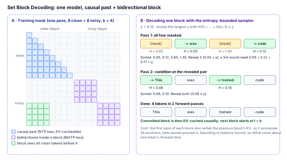
To avoid two forward passes per batch, training concatenates the clean sequence and its noised copy and uses a FlexAttention mask with three regions (panel A of the figure):
# FlexAttention mask (training time); sequence = [clean | noisy], each half_seq long
def mask_mod(b, h, q_idx, kv_idx):
    half_seq = seq_len // 2
    # 1. Causal attention among clean tokens
    is_top_left = (q_idx < half_seq) & (kv_idx < half_seq) & (kv_idx <= q_idx)
    # 2. Bidirectional attention within each noisy block
    q_blk, kv_blk = (q_idx - half_seq) // block_len, (kv_idx - half_seq) // block_len
    is_bottom_right = (q_idx >= half_seq) & (kv_idx >= half_seq) & (q_blk == kv_blk)
    # 3. A noisy block sees every clean token from earlier blocks
    is_bottom_left = (q_idx >= half_seq) & (kv_idx < half_seq) & (q_blk > (kv_idx // block_len))
    return is_top_left | is_bottom_right | is_bottom_left
Note the third region: a noisy block sees the clean tokens of earlier blocks only, exactly the context $x_{<t}$ it will have at inference time. The first block sees no clean context at all.
3. The Loss, and Why NTP Must Stay
Per training step, sample a mask rate $\tau \sim U(0, 1)$ and a block size $k \sim U(2, 16)$, then mask each position independently:
\[\hat x_i = \begin{cases} m & \text{with probability } \tau \\ x_i & \text{with probability } 1 - \tau \end{cases}\]The loss is NTP plus MATP over the masked positions of every block:
\[\mathcal{L}(x, \hat x; \theta) = \underbrace{-\sum_{t=2}^{L} \log p_\theta(x_t \mid x_{<t}\,;\,)}_{\text{NTP}} \;-\; \underbrace{\sum_{t \in T} \sum_{i=0}^{k-1} \mathbb{1}\left[\hat x_{t+i} = m\right] \log p_\theta(x_{t+i} \mid x_{<t}\,;\, \hat x_t, \dots, \hat x_{t+k-1})}_{\text{MATP}}\]with block starts $T = \lbrace 1 + \ell k \mid \ell = 0, 1, \dots, \lfloor L/k \rfloor - 1 \rbrace$.
The NTP term is not optional. In the 3B fine-tuning ablation, dropping it (training on MATP alone) leaves the NTP loss well above the baseline’s (about 2.15 vs 1.85 over the last 10% of training), and likelihood-based benchmarks (MMLU, ARC-Challenge, HellaSwag) fall by 5 to 12%: the model forgets how to be a good left-to-right model. With the joint loss, NTP loss tracks the plain NTP baseline while the model also learns block decoding.
4. Decoding: the Entropy-Bounded Sampler
SBD borrows the Entropy-Bounded (EB) Sampler from the discrete-diffusion literature. For each block:
- Start with all masks: $\hat x_{t:t+k-1} = (m, \dots, m)$.
- Run one forward pass to get logits for every masked position.
- Compute each masked position’s entropy:
- Sort masked positions by entropy, lowest first: $i_1, i_2, \dots$
- Pick the largest $s \ge 1$ with
- Sample and reveal those $s$ tokens together. Repeat from step 2 until the block is full.
- Append the block to the context; its KV entries are written causally, and decoding moves to $t + k$.
The bound in step 5 sums the entropies of all selected tokens except the most uncertain one. Intuitively, the error from sampling several tokens as if they were independent is controlled by how much uncertainty the others carry, so very confident tokens can ride along with one less certain token. At least one token is always revealed, so a block never needs more than $k$ passes. A single knob, $\gamma$, trades speed for accuracy.
Panel B of the figure walks through a 4-token block at $\gamma = 0.15$. With sorted entropies 0.05, 0.12, 0.85, 1.40, the sampler reveals two tokens ($0.05 \le \gamma$); a third would need $0.05 + 0.12 = 0.17 > \gamma$. The second pass, now conditioned on those two, is confident about the rest and finishes the block: 4 tokens in 2 forward passes.
5. Why Fewer Forward Passes Means Proportionally Less Time
The paper backs the speedup claim with a roofline model of an 8B model in FP8 on an H100 (3.35 TB/s HBM bandwidth, 1978 TFLOP/s FP8 peak):
\[\text{time} = \max\left( \frac{\text{bytes moved}}{\text{memory bandwidth}},\; \frac{\text{FLOPs}}{\text{peak FLOPs}} \right)\]At batch size 1, a single-token forward is entirely memory-bound. Going from 1 to $k = 16$ tokens per pass adds FLOPs but barely adds bytes: the weights are read once for all $k$ tokens, and once the KV cache is 1024+ tokens long, reading it dominates any per-token traffic. The modeled slowdown of a 16-token forward over a 1-token forward is only 1.004 to 1.015×.
If a block of $k$ tokens takes $\ell$ passes, the theoretical speedup is
\[\text{speedup}(\ell, k) = \frac{k \cdot \text{time}(1)}{\text{time}(2k) + (\ell - 1) \cdot \text{time}(k)}\]The first pass of each block costs $\text{time}(2k)$ because it also processes the previous block’s $k$ tokens to write their KV entries. Since $\text{time}(2k) \approx \text{time}(k) \approx \text{time}(1)$ in this regime, the reduction in forward passes $k/\ell$ carries over almost 1:1 to latency. For the underlying arithmetic, see The Economics of a Token and Efficiency in LLMs. The argument holds at small batch sizes; at large batch the GPU is closer to compute-bound and extra positions per pass are no longer free.
6. Results
Llama-3.1 8B and Qwen-3 8B base models are fine-tuned on 70B tokens of instruction, code, and math-reasoning data, once with plain NTP (baseline) and once with the SBD objective.
| Model | Method | Fewer forward passes | MATH500 | AIME25 | LiveCodeBench v6 | GSM8K | HumanEval+ | MBPP |
|---|---|---|---|---|---|---|---|---|
| Llama-3.1 8B | NTP baseline | 1.0× | 80.2 | 33.3 | 31.5 | 85.3 | 56.7 | 70.4 |
| SBD, $\gamma_{\text{low}}$ | 3.0× | 81.0 | 30.0 | 31.7 | 84.2 | 57.9 | 69.5 | |
| SBD, $\gamma_{\text{high}}$ | 3.4× | 80.4 | 23.3 | 29.9 | 84.0 | 54.9 | 67.2 | |
| Qwen-3 8B | NTP baseline | 1.0× | 86.6 | 33.3 | 36.6 | 90.1 | 69.5 | 78.0 |
| SBD, $\gamma_{\text{low}}$ | 3.2× | 85.0 | 33.3 | 37.2 | 90.1 | 66.5 | 77.5 | |
| SBD, $\gamma_{\text{high}}$ | 3.8× | 85.4 | 26.6 | 33.3 | 88.7 | 65.2 | 74.6 |
All scores are accuracy in %, from Table 1 of the paper.
- Conservative thresholds ($\gamma_{\text{low}} \in [0.1, 0.35]$) give roughly a 3× reduction (3.0 to 3.2× in the table, up to 3.9× on individual benchmarks) with accuracy close to the NTP baseline: some benchmarks go slightly up, some slightly down.
- Aggressive thresholds ($\gamma_{\text{high}} \in [0.35, 0.6]$) push the reduction up to 5.36× on LiveCodeBench, at a real accuracy cost.
- AIME25 is the sensitive one. It has only 30 problems, so each problem is 3.3 points: Llama’s 33.3 → 30.0 at $\gamma_{\text{low}}$ is one problem, but the drop to 23.3 at $\gamma_{\text{high}}$ (and 26.6 for Qwen) is three or two. Long, exact reasoning chains are where loose parallel sampling hurts first.
- Training cost: with SBD folded into SFT, about 34k iterations are needed to match the baseline’s causal performance.
7. How SBD Compares
| Speculative decoding (draft model, Medusa, EAGLE) | Masked diffusion LLMs | Set Block Decoding | |
|---|---|---|---|
| Extra components | Draft model or extra heads | None | None |
| Order of generation | Left to right; verification accepts a contiguous prefix | Any order, whole sequence | Any order within a block; blocks left to right |
| KV cache | Exact | Approximate or none | Exact (causal past) |
| Main knob | Draft design, tree shape, acceptance | Sampler schedule | $\gamma$ |
SBD sits between the two. It keeps the serving model a causal LLM with an exact KV cache, and borrows diffusion-style any-order sampling only inside the current block. That blend is close in spirit to DFlash and DSpark, which use block diffusion as the drafter for speculative decoding; SBD instead folds the block predictor into the main model and drops verification. It is also a cousin of the multi-token-prediction heads in DeepSeek-V3, without the extra heads.
Takeaways
- A causal LLM can learn block decoding by fine-tuning alone. Same architecture and weights shape, no heads or draft model; only the training objective and attention mask change.
- Keep the NTP loss. Without it, likelihood benchmarks drop 5 to 12% as the model forgets left-to-right modeling.
- Reveal by entropy, not by position. The EB sampler unmasks whichever tokens are confident, in any order, with one threshold $\gamma$ to tune.
- Memory-bound decoding makes it nearly free. A 16-token forward costs 1.004 to 1.015× a 1-token forward on an H100 at batch 1, so fewer passes translate almost 1:1 into lower latency.
- Expect about 3× at no meaningful accuracy cost, more if you accept losses; long, exact reasoning (AIME) degrades first.