Modular TTT: Composable Test-Time Training as Online Optimization
Reading notes on:
Test-Time Training (TTT) makes a sharp conceptual move: the model’s “hidden state” is no longer a fixed vector but the parameter state of a small inner learner that updates during inference. That gives sequence models a much higher-capacity memory than standard recurrences, but it also created a practical problem: every architectural tweak used to require re-deriving the whole chunkwise update rule by hand.
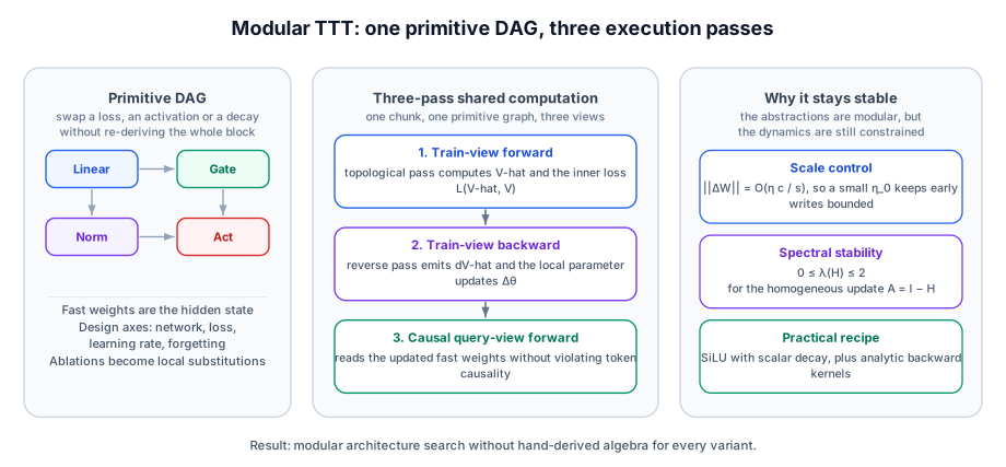
Modular TTT fixes that bottleneck. Instead of treating TTT-Linear or TTT-MLP as monolithic blocks, it factors the inner learner into reusable primitives with explicit train-time and query-time semantics. The result is not just a better TTT block. It is a cleaner way to reason about fast-weight sequence models, much like Looped Transformers separated architectural depth from compute depth, or how Engram reframed memory as an explicit retrieval system rather than a hidden-state accident.
1. Why Hard-Coded TTT Hit a Ceiling
Classical TTT variants were built as one-off derivations. Change the activation, the loss, or the decay rule, and the algebra had to be redone globally. That makes it almost impossible to answer the questions that actually matter:
- Is the gain coming from the optimization geometry or from one lucky normalization constant?
- Does a better loss help because of its statistics or because it accidentally stabilizes the write dynamics?
- Are deeper inner learners genuinely more expressive, or just harder to optimize?
Modular TTT isolates those variables. The design space is factored into four independent knobs:
- the fast-weight network itself;
- the internal loss;
- the learning-rate rule;
- the forgetting or decay mechanism.
The important consequence is methodological. Once the inner learner is written as a directed acyclic graph of primitives, architectural ablations stop being global rewrites and become local substitutions.
2. The Core Mechanism: One DAG, Three Passes
Let the inner learner be a DAG $G = (V, E)$ whose nodes are primitive operations $\phi_j$. Modular TTT assigns each primitive three views:
| Primitive | Train Forward | Train Backward | Query View |
|---|---|---|---|
| Linear | $\hat{V} = K W$ | $dW = \hat{K}^T d\hat{V}$ | $O = QW - \text{Tril}(QK^T \odot M)d\hat{V}$ |
| Gate | $\hat{V} = K \odot W$ | $dW = \sum(\hat{K} \odot d\hat{V})$ | $O = QW - Q \odot \text{cumsum}(\hat{K} \odot d\hat{V})$ |
| Norm | $\hat{v} = k / \sigma$ | $dk = (d\hat{v} - c\hat{v}) / \sigma$ | standard normalization semantics |
| Act | $\hat{V} = f(K)$ | $dK = d\hat{V} \odot f’(K)$ | $O = f(R)$ |
Execution happens in three strict passes over each chunk:
- Train-view forward. Compute $\hat{V}$ topologically so the inner loss $L(\hat{V}, V)$ can be evaluated.
- Train-view backward. Traverse the graph in reverse to get $d\hat{V}$ and the local parameter updates $\Delta \theta_j$.
- Causal query-view forward. Read from the updated fast weights while preserving causality.
For a linear primitive, writing the scaled key as $\hat{k}_t = \eta_t k_t$, the recurrence is
\[W_t = W_{t-1} - \hat{k}_t^T d\hat{v}_t.\]Unrolling the recurrence over a chunk gives
\[W_t = W_{\text{start}} - \sum_{s=1}^t \hat{k}_s^T d\hat{v}_s,\]so the readout at position $t$ is
\[o_t = q_t W_t = q_t W_{\text{start}} - \sum_{s=1}^t (q_t \hat{k}_s^T) d\hat{v}_s.\]Stacking the chunk into matrices produces the key identity:
\[O = QW_{\text{start}} - \text{Tril}(Q \hat{K}^T)\, d\hat{V}, \qquad W_{\text{end}} = W_{\text{start}} - \hat{K}^T d\hat{V}.\]This is the whole point of the framework. Once each primitive exports these three semantics, the chunkwise computation graph can be assembled automatically instead of re-derived by hand.
3. What the Math Says About Stability
3.1 Scale control is mostly a learning-rate problem
The chunk update norm obeys
\[\lVert \Delta W \rVert_F = O(\eta c / s),\]where $c$ is chunk size and $s$ is the loss-scaling constant. If $s = 1$, the update grows linearly with chunk length. Modular TTT gets around this with small-lr initialization, using $\eta_0 \approx 10^{-3}$ so that even at large chunk sizes the initial update remains $O(1)$ instead of exploding.
3.2 Spectrum control is the real stability condition
Define
\[A = I - H, \qquad H = K^T \text{diag}(\eta) K.\]The homogeneous update is stable only if every eigenvalue of $A$ stays inside the unit disk, which reduces to
\[0 \le \lambda_i(H) \le 2.\]Since $H \preceq \eta_0 K^T K$ when $\eta_t \le \eta_0$, it is enough to keep
\[\lambda_{\max}(H) \le \eta_0 \lVert K \rVert_2^2\]small. The practical message is simple: most TTT instability is not mysterious. It is spectral blow-up in disguise.
3.3 Not every loss is usable as a write signal
Modular TTT’s ablations explain why L1 and RMSE underperform. Both throw away the residual magnitude:
- L1 depends only on $\text{sign}(R)$.
- RMSE normalizes by $\lVert R \rVert_F$.
So for any scale factor $a > 0$, the gradient of $aR$ looks the same as the gradient of $R$. That removes information about how wrong the model is. In a fast-weight memory, that amplitude is exactly what determines the strength of the write. MSE and inner-product losses keep that scale information and behave much better.
3.4 Deeper memories are hard for a structural reason
For a depth-two learner $Y = XW_1W_2$, the update to factor $W_j$ takes the form
\[\Delta W_j = A_{j-1}^T D B_{j+1}^T.\]The functional mapping can stay unchanged under a rescaling
\[W_1W_2 = (cW_1)(c^{-1}W_2),\]but the update geometry does not stay invariant. The optimization now depends on the factorization itself, not only on the realized matrix product. That is the “deep memory barrier”: deeper TTT learners add representational freedom, but also inject a non-convex factor-coupling problem into every online update.
3.5 Zero initialization is a trap for $L \ge 2$
If all factors in a deep learner are initialized to zero, then either the upstream activations or the downstream factors vanish, and the gradient is exactly zero. A single-layer learner avoids this because its update is simply $\Delta W = K^T D$, which is generically non-zero.
4. What Actually Helped in Practice
The ablations are refreshingly concrete.
4.1 Simple pointwise activations beat fancy structure
GELU and SiLU consistently help because they gate the write signal coordinate-wise without introducing difficult factor interactions. In contrast, RMSNorm is fragile: its gradient contains a $1 / \sigma(z)$ amplification term, so what often looks like “better normalization” is really just a fight against gradient blow-up by increasing $\epsilon$.
4.2 Forgetting needs to be cheap
Weight decay matters because stale context has to be erased. The best-quality option is vector decay, which forgets feature-wise, but it costs about a 25% throughput penalty and roughly 3 GB of extra peak memory. The paper’s practical recommendation is scalar decay: most of the quality gain at almost none of the systems cost.
4.3 Some familiar FFN tricks do not survive the online-update regime
SwiGLU and residual inner learners failed to beat a Linear + SiLU baseline. That is not because they lack expressive power; it is because branch interactions and factor coupling make one-step online optimization much harder than ordinary feed-forward training.
4.4 The systems work is real, not cosmetic
Modular TTT uses custom analytic backward operators that compile cleanly with torch.compile. The payoffs are material:
- 1.65x speedup for the linear primitive over
torch.autograd.grad; - 2.62x speedup for the normalization primitive;
- normalization memory reduced from 31.3 MB to 19.3 MB.
At the end-to-end level, Modular TTT reports 2.2x to 3.3x throughput gains over the official TTT-Linear and TTT-MLP baselines at the 160M scale, while still remaining competitive with Gated DeltaNet and LLaMA-style baselines at 1.45B scale on 100B tokens.
4.5 Long context is better, but not solved
The framework stays stable past the 4K training context and reaches 8K without sharp loss degradation. But on retrieval-style evaluations such as RULER and Needle-in-a-Haystack, it still trails full attention, especially at long context. Modular TTT improves the design space of fast-weight models; it does not erase the recall advantage of explicit attention.
Takeaways
- The real contribution is modularity, not one more TTT block. Turning TTT into a graph of primitives makes the design space searchable instead of artisanal.
- Stability is mostly spectral geometry. Small initialization and bounded effective Hessians matter more than cosmetic architecture changes.
- Write signals need magnitude information. L1 and RMSE look attractive as robust losses, but they erase the very amplitude information a fast-weight memory needs.
- Shallow inner learners are not a historical accident. The failure of deeper memories follows from factor-coupled optimization, not from insufficient engineering effort.
- The systems side finally caught up. Analytic backward kernels and compiled execution are what make TTT feel like a viable sequence-modeling family rather than a theoretical curiosity.